Perform PK/PD Modeling and Simulation to Guide Dosing Strategy for Antibiotics
This example shows how to perform a Monte Carlo simulation of a pharmacokinetic/pharmacodynamic (PK/PD) model for an antibacterial agent. This example is adapted from Katsube et al. [1] This example also shows how to use the SimBiology® SimFunction object to perform parameter scans in parallel.
This example requires Statistics and Machine Learning Toolbox™. The performance can be improved if you have the Parallel Computing Toolbox™ software.
Background
Katsube et al. [1] used a PK/PD modeling and simulation approach to determine the most effective dosage regimens for doripenem, a carbapenem antibiotic. The objectives of their study were:
Develop a PK/PD model to describe the antibacterial effect of doripenem against several Pseudomonas aeruginosa strains
Use Monte Carlo simulations to compare the efficacy of four common antibiotic dosage regimes, and to determine the most effective dosing strategy
Investigate the effect of renal function on the antibacterial efficacy of the treatments
In this example, we will implement the antibacterial PK/PD model developed by Katsube et al. [1] in SimBiology®, and replicate the results of the Monte Carlo simulation described in their work.
References
[1] T. Katsube, Y. Yano, T. Wajima, Y. Yamano and M. Takano. Pharmacokinetic/pharmacodynamic modeling and simulation to determine effective dosage regimens for doripenem. Journal of Pharmaceutical Sciences (2010) 99(5), 2483-91.
PK/PD Model
Katsube et al. assumed a two-compartment infusion model with linear elimination from the central compartment to describe the pharmacokinetics of the doripenem. For the bacterial growth model, they assumed that the total bacterial population is comprised of drug-susceptible growing cells and drug-insensitive resting cells. The antibacterial effect of the drug was included in the killing rate of the bacteria via a simple Emax type model:
![$$ Killing Rate = \frac{Kmax*[Drug]*[Growing]}{KC50 + [Drug]} $$](../../examples/simbio/win64/antibioticdemo_eq16197705998259887470.png)
where [Drug] is the concentration (ug/ml) of the drug in the central compartment, and [Growing] is the count of the growing bacterial population in CFU/ml (CFU = Colony Forming Units). Kmax is the maximal killing rate constant (1/hour) and KC50 is the Michaelis-Menten rate constant (ug/ml).
A graphical view of the SimBiology implementation of the model is shown below.

% Load model
sbioloadproject('AntibacterialPKPD.sbproj', 'm1') ;
Dosage Regimens
Katsube et al. simulated the model using four common antibiotic dosage strategies.
250 mg two times a day (b.i.d.)
250 mg three times a day (t.i.d.)
500 mg two times a day (b.i.d.)
500 mg three times a day (t.i.d.)
Infusion dosing was used in all four dosages regimens, and infusion time was set to 30 minutes. In SimBiology, these dosage regimens have been implemented as dose objects.
% Select dose objects in the model
doseNames = {'250 mg bid', '250 mg tid', '500 mg bid', '500 mg tid'};
for iDoseGrp = 1:length(doseNames)
    doseRegimens(iDoseGrp) = sbioselect(m1, 'Name', doseNames{iDoseGrp}) ;
end
Description of the Virtual Population
A virtual population of individuals was generated based on the distribution of demographic variables and PK/PD parameters. The type of distribution and the values of the distribution parameters were based on data from earlier clinical trials of doripenem conducted in Japan.
Note: In [1], 5,000 virtual patients were simulated in each dosage group. In this example, we will use 1,000 patients in each group. To simulate a different population size, change the value of nPatients below.
% Setup
nPatients    = 1000         ; % Number of patients per dosage group
nDoseGrps    = 4            ; % Number of tested dosage regimens
Distribution of Demographic Variables:
Weight (Wt) and age (Age) were sampled from a normal distribution with a mean of 51.6 kg and 71.8 years, respectively, and a standard deviation of 11.8 kg and 11.9 years, respectively. 26% of the population was assumed to be female. Serum creatinine levels (Scr) were sampled from a lognormal distribution with the typical value (geometric mean) of 0.78 mg/dL, and coefficient of variation (CV) of 32.8%. The creatinine clearance rates (CrCL) were calculated using the Cockcroft-Gault equation.
The inputs to the lognrnd function are the mean (mu) and standard deviation (sigma) of the associated normal distribution. Here and throughout the example, mu and sigma were calculated from the reported typical value and coefficient of variation of the lognormal distribution. You can use the following definitions to calculate them. See the lognstat documentation for more information.
mu    = @(m,v) log(m^2/sqrt(v+m^2));
sigma = @(m,v) sqrt(log(v/m^2+1));
m     = @(typicalValue) typicalValue;
v     = @(typicalValue,CV) typicalValue^2*CV^2;

% Patient demographics
rng('default');
Wt        = normrnd(51.6, 11.8, nPatients , nDoseGrps )   ; % units: kg
Age       = normrnd(71.8, 11.9, nPatients , nDoseGrps )   ; % units: years
Scr_mu    =    mu(m(0.78), v(0.78,0.328));
Scr_sigma = sigma(m(0.78), v(0.78,0.328));
Scr       = lognrnd(Scr_mu, Scr_sigma, nPatients , nDoseGrps )   ; % units: ml/minute
% Gender ratio
id        = 1:nPatients*nDoseGrps                            ;
idFemale  = randsample(id , round(0.26*nDoseGrps*nPatients)) ; % 26% Female
Creatinine Clearance (using Cockcroft-Gault equation)
CrCL            = (140 - Age).*Wt./(Scr*72)                 ; % units: ml/minute
CrCL(idFemale)  = CrCL(idFemale)*0.85                       ; % multiply by 0.85 for females
Distribution of Pharmacokinetic (PK) parameters:
PK parameters, Central, k12, and k21, were sampled from a lognormal distribution with typical values of 7.64 liters, 1.59 1/hour and 2.26 1/hour, respectively, and a 20% coefficient of variation (CV). Central is the distribution volume of the central compartment, and k12 and k21 are transfer rate constants between the Central and the Peripheral compartments.
Central_mu    =    mu(m(7.64), v(7.64,0.20));
Central_sigma = sigma(m(7.64), v(7.64,0.20));
k12_mu        =    mu(m(1.59), v(1.59,0.20));
k12_sigma     = sigma(m(1.59), v(1.59,0.20));
k21_mu        =    mu(m(2.26), v(2.26, 0.2));
k21_sigma     = sigma(m(2.26), v(2.26, 0.2));

Central = lognrnd(Central_mu , Central_sigma, nPatients , nDoseGrps); % units: liter
k12     = lognrnd(k12_mu, k12_sigma, nPatients , nDoseGrps)         ; % units: 1/hour
k21     = lognrnd(k21_mu, k21_sigma, nPatients , nDoseGrps)         ; % units: 1/hour
The drug clearance rate, CL, was assumed to depend linearly on the creatinine clearance rate via the following equation:

where  is the additive residual error sampled from a normal distribution with a mean of 0 ml/minute and standard deviation of 22 ml/minute.
CL = 1.07*CrCL + 45.6 + normrnd(0,22,nPatients,nDoseGrps); % units: ml/minute
Distribution of Pharmacodynamic (PD) parameters:
Growing-to-resting transformation rate constants, k1 and k2, were sampled from a lognormal distribution with typical value of 5.59e-5 and 0.0297 1/hour, respectively, each with a CV of 20%. Kmax was sampled from a lognormal distribution with a typical value of 3.5 1/hour and 15.9% CV.
k1_mu      =    mu(m(5.59e-5), v(5.59e-5, 0.2));
k1_sigma   = sigma(m(5.59e-5), v(5.59e-5, 0.2));
k2_mu      =    mu(m(0.0297) , v(0.0297, 0.2));
k2_sigma   = sigma(m(0.0297) , v(0.0297, 0.2));
Kmax_mu    =    mu(m(3.50)   , v(3.50, 0.159));
Kmax_sigma = sigma(m(3.50)   , v(3.50, 0.159));

k1   = lognrnd(k1_mu, k1_sigma, nPatients , nDoseGrps)     ; % units: 1/hour
k2   = lognrnd(k2_mu, k2_sigma, nPatients , nDoseGrps)     ; % units: 1/hour
Kmax = lognrnd(Kmax_mu, Kmax_sigma, nPatients , nDoseGrps) ; % units: 1/hour
Katsube et al. assumed that values k1, k2 and Kmax were independent of the bacterial strain being treated. The value of Beta, the net growth rate constant, was fixed at 1.5 1/hour.
Based on experiments with several strains, the authors concluded that the value of KC50 was linearly dependent on the minimum inhibition concentration (MIC) of bacterial strain via the following equation.

where is the additive residual error sampled from a normal distribution with a mean of 0 and standard deviation of 1.06 ug/ml. In the simulation, the MIC values were sampled from a discrete distribution, and the KC50 value was calculated for the selected MIC using the above equation.
% Discrete distribution of MIC values based on 71 P. aeruginosa strains
micValue  = [0.0625, 0.125, 0.25, 0.5 , 1 , 2 , 4 , 8 , 16 , 32 ] ;
micFreq   = [   5  ,    8 ,  9  , 14  , 7 , 8 , 9 , 5 , 2  , 4  ] ;

% Sample MIC values from a discrete distribution using randsample
MIC = nan(nPatients, nDoseGrps) ; % preallocate
for iDoseGrp = 1:nDoseGrps
    MIC(:, iDoseGrp) = randsample(micValue , nPatients, true , micFreq);
end

KC50 = exp(-1.91 + 0.898*log(MIC) + 1.06*randn(nPatients , nDoseGrps)) ; % units: microgram/milliliter
Simulation Setup & Design
Create a SimFunction object that lets you perform model simulations and parameter scans in parallel. In this example, you will vary 8 parameters, Central, k12, k21, CL, k1, k2, Kmax, and KC50. Select the growing and resting bacterial counts, Growing and Resting, as responses, that is, simulation results that you want to observe while varying those input parameters.
Select the parameters to vary.
params = {'Central', 'k12', 'k21', 'CL', 'k1', 'k2', 'Kmax', 'KC50'};
Select the responses.
observables = {'[Bacterial Growth Model].Growing',...
               '[Bacterial Growth Model].Resting'};
Set up a template dose.
tempdose = sbiodose('dose');
tempdose.Target = 'Central.Drug';
tempdose.AmountUnits = 'milligram';
tempdose.TimeUnits = 'hour';
tempdose.DurationParameterName = 'TDose';
Create a SimFunction object. Set UseParallel to true to enable parallel computing.
simfunc = createSimFunction(m1,params,observables,tempdose,'UseParallel',true);
Create an input matrix phi for each dosage group.
phi = cell(1,nDoseGrps);
for i = 1:nDoseGrps
    phi{i} = [Central(:,i),k12(:,i),k21(:,i), ...
              CL(:,i), k1(:,i), k2(:,i), ...
              Kmax(:,i), KC50(:,i)];
end
Cluster Computing
This example uses the local cluster profile that is pre-configured to your local machine. You can also search for other MATLAB® Parallel Server™ clusters that are running on Amazon EC2®. On the Home tab in the Environment section, select Parallel > Discover Clusters. To access these clusters, you must provide your MathWorks® Account login information. For details, see Discover Clusters and Use Cluster Profiles (Parallel Computing Toolbox).
Create a parallel pool if none exists.
if isempty(gcp)
    parpool;
end
Starting parallel pool (parpool) using the 'Processes' profile ...
Connected to parallel pool with 4 workers.
For all dosage scenarios, the model was simulated until t = 2 weeks from the time of the first dose. Total bacterial count, CFU, was sampled every 24 hours (once a day) for the entire duration of the dosage regimen.
tObs      = 0:24:336       ; % hour
nTPoints  = length(tObs)   ; % Number of sampling points
Monte Carlo Simulation of Patients with Severe Infection
The antibacterial efficacy of a drug can be measured using different PK/PD indices. Katsube et al. set the criterion for bacterial elimination at log10(CFU) < 0, where CFU is the total bacterial count. The efficacy of each dose regimen was measured as the fraction of the population that achieved the success criteria in the dosage group. This efficacy metric, Pr{log10(CFU) < 0}, was tracked as a function of time for each dosage group.
In their simulation studies, the authors investigated the efficacy of the dosage regimens on two classes of patients:
Moderate infection (Initial bacterial count = 1e4 CFU/ml)
Severe infection (Initial bacterial count = 1e7 CFU/ml)
In this example, we will replicate the results for the severe infection case only. Note that you can easily simulate the other scenario, patients with moderate infection, by changing the initial amount of bacterial count (the Growing species), in the model to 1e4 CFU/ml.
% Preallocate
cfu          = nan(nTPoints,nPatients);
log10CFU     = cell(1,nDoseGrps) ;

for i = 1:nDoseGrps
    disp(['Simulating group ', num2str(i),'...'])

    % Get the dose table directly from an existing dose object for each
    % dosing regimen.
    doseTable = getTable(doseRegimens(i));

    % Simulate
    simdata = simfunc(phi{i},[],doseTable,tObs);

    % Sum of growing and resting bacterial counts for each patient
    for j = 1:nPatients
       cfu(:,j) = sum(simdata(j).Data,2);
    end
    % Store log-transformed counts for each dose group.
    log10CFU{i} = log10(cfu);
end

% Save results
log10CFU_250bid = log10CFU{1} ;
log10CFU_250tid = log10CFU{2} ;
log10CFU_500bid = log10CFU{3} ;
log10CFU_500tid = log10CFU{4} ;
Simulating group 1...
Simulating group 2...
Simulating group 3...
Simulating group 4...
Shut down the parallel pool.
delete(gcp('nocreate'));
Parallel pool using the 'Processes' profile is shutting down.
Time Course Profiles of Bacterial Counts
We plot the median (in red) and percentile (shaded) profiles of the log10(CFU) levels for all four dosage regimens. Observe that in all four groups, the median time course profile shows that bacterial eradication is complete before the end of the treatment period (336 hours). However, it is evident from the higher percentile profiles that the treatments are not successful for all patients. The 95th and 90th percentile profiles also indicate that dosing a lower amount with a higher frequency (250 tid) is more effective than less frequent dosing with higher amount (500 bid).
hax1(1) = subplot(2,2,1)
plotCFUCount(tObs, log10CFU_250bid, 'a. Dose 250 bid' )
hax1(2) = subplot(2,2,2)
plotCFUCount(tObs, log10CFU_250tid, 'b. Dose 250 tid' )
hax1(3) = subplot(2,2,3)
plotCFUCount(tObs, log10CFU_500bid, 'c. Dose 500 bid' )
hax1(4) = subplot(2,2,4)
plotCFUCount(tObs, log10CFU_500tid, 'd. Dose 500 tid' )

% Link subplot axes
linkaxes(hax1)
hax1 =

  Axes with properties:

             XLim: [0 1]
             YLim: [0 1]
           XScale: 'linear'
           YScale: 'linear'
    GridLineStyle: '-'
         Position: [0.1300 0.5838 0.3347 0.3412]
            Units: 'normalized'

  Use GET to show all properties


hax1 =

  1×2 Axes array:

    Axes    Axes


hax1 =

  1×3 Axes array:

    Axes    Axes    Axes


hax1 =

  1×4 Axes array:

    Axes    Axes    Axes    Axes

Effect of Renal Function on Antibacterial Activity
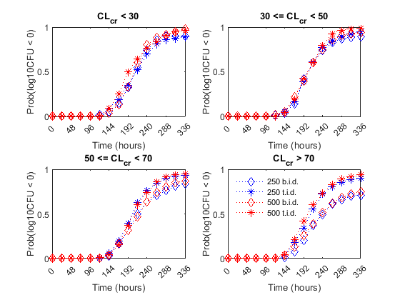
Finally, the authors compared the efficacy profiles of the dosages regimens as a function of the renal function. They classified the patients into four renal function groups based on the creatinine clearance rates (CrCL):
Creatinine Clearance Group 1:
CrCL< 30Creatinine Clearance Group 2: 30 <=
CrCL< 50Creatinine Clearance Group 3: 50 <=
CrCL< 70Creatinine Clearance Group 4:
CrCL>= 70
The next figure shows the effect of renal function (creatinine clearance rate) on the antibacterial efficacy of the four dosage regimens. Observe that in the normal renal function group (CrCL >= 70), the efficacy profiles of the four treatment strategies are significantly different from each other. In this case, the 500 mg t.i.d. dose is much more effective than the other regimens. In contrast, simulations involving patients with renal dysfunction (CrCL < 30 and 30 <= CrCL < 50), we don't see much difference between the treatment groups. This indicates that for patients with a renal dysfunction, a less intense or less frequent dosing strategy would work almost as well as a dosing strategy with higher frequency or dosing amount.
% Preallocate
idCrCLGrp   = false(nPatients, nDoseGrps) ;

% Line Style
ls = {'bd:', 'b*:', 'rd:', 'r*:'} ;

titleStr = {'CL_c_r < 30'           , ...
            '30 <= CL_c_r < 50'     , ...
            '50 <= CL_c_r < 70'     , ...
            'CL_c_r > 70'            };

f = figure;
f.Color = 'w'

for iCrCLGrp = 1:4 % Creatinine Clearance Groups

    hax2(iCrCLGrp) = subplot(2,2, iCrCLGrp) ;
    title( titleStr{iCrCLGrp}   ) ;
    ylabel('Prob(log10CFU < 0)' ) ;
    xlabel('Time (hours)'       ) ;

end

% Set axes properties
set(hax2,   'XTick'        , 0:48:336      , ...
            'XTickLabel'   , 0:48:336      , ...
            'Ylim'         , [0 1]         , ...
            'Xlim'         , [0 336]       , ...
            'NextPlot'     , 'add'         , ...
            'Box'          , 'on'          );

% Plot results by renal function group:
for iDoseGrp = 1:nDoseGrps

    % Extract indices for renal function
    idCrCLGrp(:, 1) = CrCL(:,iDoseGrp) < 30                                    ;
    idCrCLGrp(:, 2) = CrCL(:,iDoseGrp) >= 30 & CrCL(:,iDoseGrp) < 50           ;
    idCrCLGrp(:, 3) = CrCL(:,iDoseGrp) >= 50 & CrCL(:,iDoseGrp) < 70           ;
    idCrCLGrp(:, 4) = CrCL(:,iDoseGrp) >= 70                                   ;

    for iCrCLGrp = 1:4 % Creatinine Clearance Groups

        % Calculate probability
        Pr = sum( ( log10CFU{iDoseGrp}(:, idCrCLGrp(:, iCrCLGrp)') < 0) , 2 )/sum(idCrCLGrp(:,iCrCLGrp)) ;

        % Plot
        plot(hax2(iCrCLGrp), tObs, Pr , ls{iDoseGrp}, 'MarkerSize', 7)
    end

end

legend(hax2(4), {'250 b.i.d.', '250 t.i.d.', '500 b.i.d.', '500 t.i.d.'} )
legend location NorthWest
legend boxoff

linkaxes(hax2)
f =

  Figure (1) with properties:

      Number: 1
        Name: ''
       Color: [1 1 1]
    Position: [1256 1106 560 420]
       Units: 'pixels'

  Use GET to show all properties
You can also select a web site from the following list:
Americas
- América Latina (Español)
- Canada (English)
- United States (English)
Europe
- Belgium (English)
- Denmark (English)
- Deutschland (Deutsch)
- España (Español)
- Finland (English)
- France (Français)
- Ireland (English)
- Italia (Italiano)
- Luxembourg (English)
- Netherlands (English)
- Norway (English)
- Österreich (Deutsch)
- Portugal (English)
- Sweden (English)
- Switzerland
- United Kingdom (English)