Main Content

pidtune

PID tuning algorithm for linear plant model

Syntax

C = pidtune(sys,type)
C = pidtune(sys,C0)
C = pidtune(sys,type,wc)
C = pidtune(sys,C0,wc)
C = pidtune(sys,...,opts)
[C,info] = pidtune(...)

Description

C = pidtune(sys,type) designs a PID controller of type type for the plant sys. If type specifies a one-degree-of-freedom (1-DOF) PID controller, then the controller is designed for the unit feedback loop as illustrated:

If type specifies a two-degree-of-freedom (2-DOF) PID controller, then pidtune designs a 2-DOF controller as in the feedback loop of this illustration:

pidtune tunes the parameters of the PID controller C to balance performance (response time) and robustness (stability margins).

C = pidtune(sys,C0) designs a controller of the same type and form as the controller C0. If sys and C0 are discrete-time models, C has the same discrete integrator formulas as C0.

C = pidtune(sys,type,wc) and C = pidtune(sys,C0,wc) specify a target value wc for the first 0 dB gain crossover frequency of the open-loop response.

C = pidtune(sys,...,opts) uses additional tuning options, such as the target phase margin. Use pidtuneOptions to specify the option set opts.

[C,info] = pidtune(...) returns the data structure info, which contains information about closed-loop stability, the selected open-loop gain crossover frequency, and the actual phase margin.

Input Arguments

sys

Single-input, single-output dynamic system model of the plant for controller design. sys can be:

  • Any type of SISO dynamic system model, including Numeric LTI models and identified models. If sys is a tunable or uncertain model, pidtune designs a controller for the current or nominal value of sys.

  • A continuous- or discrete-time model.

  • Stable, unstable, or integrating. A plant with unstable poles, however, might not be stabilizable under PID control.

  • A model that includes any type of time delay. A plant with long time delays, however, might not achieve adequate performance under PID control.

  • An array of plant models. If sys is an array, pidtune designs a separate controller for each plant in the array.

If the plant has unstable poles, and sys is one of the following:

  • A frd model

  • A ss model with internal time delays that cannot be converted to I/O delays

you must use pidtuneOptions to specify the number of unstable poles in the plant, if any.

type

Controller type of the controller to design, specified as a character vector. The term controller type refers to which terms are present in the controller action. For example, a PI controller has only a proportional and an integral term, while a PIDF controller contains proportional, integrator, and filtered derivative terms. type can take the values summarized below. For more detailed information about these controller types, see PID Controller Types for Tuning

1-DOF Controllers

  • 'P' — Proportional only

  • 'I' — Integral only

  • 'PI' — Proportional and integral

  • 'PD' — Proportional and derivative

  • 'PDF' — Proportional and derivative with first-order filter on derivative term

  • 'PID' — Proportional, integral, and derivative

  • 'PIDF' — Proportional, integral, and derivative with first-order filter on derivative term

2-DOF Controllers

  • 'PI2' — 2-DOF proportional and integral

  • 'PD2' — 2-DOF proportional and derivative

  • 'PDF2' — 2-DOF proportional and derivative with first-order filter on derivative term

  • 'PID2' — 2-DOF proportional, integral, and derivative

  • 'PIDF2' — 2-DOF proportional, integral, and derivative with first-order filter on derivative term

For more information about 2-DOF PID controllers generally, see Two-Degree-of-Freedom PID Controllers.

2-DOF Controllers with Fixed Setpoint Weights

  • 'I-PD' — 2-DOF PID with b = 0, c = 0

  • 'I-PDF' — 2-DOF PIDF with b = 0, c = 0

  • 'ID-P' — 2-DOF PID with b = 0, c = 1

  • 'IDF-P' — 2-DOF PIDF with b = 0, c = 1

  • 'PI-D' — 2-DOF PID with b = 1, c = 0

  • 'PI-DF' — 2-DOF PIDF with b = 1, c = 0

For more detailed information about fixed-setpoint-weight 2-DOF PID controllers, see PID Controller Types for Tuning.

Controller Form

When you use the type input, pidtune designs a controller in parallel (pid or pid2) form. Use the input C0 instead of type if you want to design a controller in standard (pidstd or pidstd2) form.

If sys is a discrete-time model with sample time Ts, pidtune designs a discrete-time controller with the same Ts. The controller has the ForwardEuler discrete integrator formula for both integral and derivative actions. Use the input C0 instead of type if you want to design a controller having a different discrete integrator formula.

For more information about PID controller forms and formulas, see:

C0

PID controller setting properties of the designed controller, specified as a pid, pidstd, pid2, or pidstd2 object. If you provide C0, pidtune:

  • Designs a controller of the type represented by C0.

  • Returns a pid controller, if C0 is a pid controller.

  • Returns a pidstd controller, if C0 is a pidstd controller.

  • Returns a 2-DOF pid2 controller, if C0 is a pid2 controller.

  • Returns a 2-DOF pidstd2 controller, if C0 is a pidstd2 controller.

  • Returns a controller with the same Iformula and Dformula values as C0, if sys is a discrete-time system. See the pid, pid2, pidstd, and pidstd2 reference pages for more information about Iformula and Dformula.

wc

Target value for the 0 dB gain crossover frequency of the tuned open-loop response. Specify wc in units of radians/TimeUnit, where TimeUnit is the time unit of sys. The crossover frequency wc roughly sets the control bandwidth. The closed-loop response time is approximately 1/wc.

Increase wc to speed up the response. Decrease wc to improve stability. When you omit wc, pidtune automatically chooses a value, based on the plant dynamics, that achieves a balance between response and stability.

opts

Option set specifying additional tuning options for the pidtune design algorithm, such as target phase margin or design focus. Use pidtuneOptions to create opts.

Output Arguments

C

Controller designed for sys. If sys is an array of linear models, pidtune designs a controller for each linear model and returns an array of PID controllers.

Controller form:

  • If the second argument to pidtune is type, C is a pid or pid2 controller.

  • If the second argument to pidtune is C0:

    • C is a pid controller, if C0 is a pid object.

    • C is a pidstd controller, if C0 is a pidstd object.

    • C is a pid2 controller, if C0 is a pid2 object.

    • C is a pidstd2 controller, if C0 is a pidstd2 object.

Controller type:

  • If the second argument to pidtune is type, C generally has the specified type.

  • If the second argument to pidtune is C0, C generally has the same type as C0.

In either case, however, where the algorithm can achieve adequate performance and robustness using a lower-order controller than specified with type or C0, pidtune returns a C having fewer actions than specified. For example, C can be a PI controller even though type is 'PIDF'.

Time domain:

  • C has the same time domain as sys.

  • If sys is a discrete-time model, C has the same sample time as sys.

  • If you specify C0, C has the same Iformula and Dformula as C0. If no C0 is specified, both Iformula and Dformula are Forward Euler. See the pid, pid2, pidstd, and pidstd2 reference pages for more information about Iformula and Dformula.

If you specify C0, C also obtains model properties such as InputName and OutputName from C0. For more information about model properties, see the reference pages for each type of dynamic system model.

info

Data structure containing information about performance and robustness of the tuned PID loop. The fields of info are:

  • Stable — Boolean value indicating closed-loop stability. Stable is 1 if the closed loop is stable, and 0 otherwise.

  • CrossoverFrequency — First 0 dB crossover frequency of the open-loop system C*sys, in rad/TimeUnit, where TimeUnit is the time units specified in the TimeUnit property of sys.

  • PhaseMargin — Phase margin of the tuned PID loop, in degrees.

If sys is an array of plant models, info is an array of data structures containing information about each tuned PID loop.

Examples

collapse all

This example shows how to design a PID controller for the plant given by:

sys=1(s+1)3.

As a first pass, create a model of the plant and design a simple PI controller for it.

sys = zpk([],[-1 -1 -1],1); 
[C_pi,info] = pidtune(sys,'PI')
C_pi =
 
             1 
  Kp + Ki * ---
             s 

  with Kp = 1.14, Ki = 0.454
 
Continuous-time PI controller in parallel form.
info = struct with fields:
                Stable: 1
    CrossoverFrequency: 0.5205
           PhaseMargin: 60.0000

C_pi is a pid controller object that represents a PI controller. The fields of info show that the tuning algorithm chooses an open-loop crossover frequency of about 0.52 rad/s.

Examine the closed-loop step response (reference tracking) of the controlled system.

T_pi = feedback(C_pi*sys, 1);
step(T_pi)

Figure contains an axes object. The axes object contains an object of type line. This object represents T\_pi.

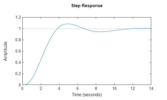
To improve the response time, you can set a higher target crossover frequency than the result that pidtune automatically selects, 0.52. Increase the crossover frequency to 1.0.

[C_pi_fast,info] = pidtune(sys,'PI',1.0)
C_pi_fast =
 
             1 
  Kp + Ki * ---
             s 

  with Kp = 2.83, Ki = 0.0495
 
Continuous-time PI controller in parallel form.
info = struct with fields:
                Stable: 1
    CrossoverFrequency: 1
           PhaseMargin: 43.9973

The new controller achieves the higher crossover frequency, but at the cost of a reduced phase margin.

Compare the closed-loop step response with the two controllers.

T_pi_fast = feedback(C_pi_fast*sys,1);
step(T_pi,T_pi_fast)
axis([0 30 0 1.4])
legend('PI','PI,fast')

Figure contains an axes object. The axes object contains 2 objects of type line. These objects represent PI, PI,fast.

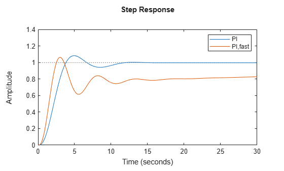
This reduction in performance results because the PI controller does not have enough degrees of freedom to achieve a good phase margin at a crossover frequency of 1.0 rad/s. Adding a derivative action improves the response.

Design a PIDF controller for Gc with the target crossover frequency of 1.0 rad/s.

[C_pidf_fast,info] = pidtune(sys,'PIDF',1.0)
C_pidf_fast =
 
             1            s    
  Kp + Ki * --- + Kd * --------
             s          Tf*s+1 

  with Kp = 2.72, Ki = 0.985, Kd = 1.72, Tf = 0.00875
 
Continuous-time PIDF controller in parallel form.
info = struct with fields:
                Stable: 1
    CrossoverFrequency: 1
           PhaseMargin: 60.0000

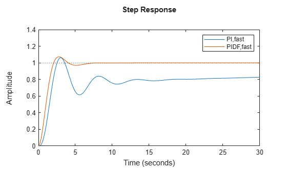
The fields of info show that the derivative action in the controller allows the tuning algorithm to design a more aggressive controller that achieves the target crossover frequency with a good phase margin.

Compare the closed-loop step response and disturbance rejection for the fast PI and PIDF controllers.

T_pidf_fast =  feedback(C_pidf_fast*sys,1);
step(T_pi_fast, T_pidf_fast);
axis([0 30 0 1.4]);
legend('PI,fast','PIDF,fast');

Figure contains an axes object. The axes object contains 2 objects of type line. These objects represent PI,fast, PIDF,fast.

You can compare the input (load) disturbance rejection of the controlled system with the fast PI and PIDF controllers. To do so, plot the response of the closed-loop transfer function from the plant input to the plant output.

S_pi_fast = feedback(sys,C_pi_fast);
S_pidf_fast = feedback(sys,C_pidf_fast);
step(S_pi_fast,S_pidf_fast);
axis([0 50 0 0.4]);
legend('PI,fast','PIDF,fast');

Figure contains an axes object. The axes object contains 2 objects of type line. These objects represent PI,fast, PIDF,fast.

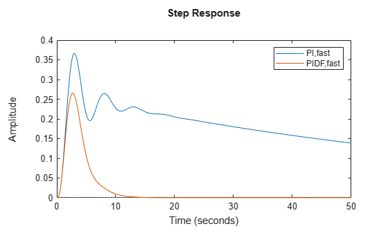
This plot shows that the PIDF controller also provides faster disturbance rejection.

Design a PID controller in standard form for the following plant.

sys=1(s+1)3

To design a controller in standard form, use a standard-form controller as the C0 argument to pidtune.

sys = zpk([],[-1 -1 -1],1);
C0 = pidstd(1,1,1); 
C = pidtune(sys,C0)
C =
 
             1      1          
  Kp * (1 + ---- * --- + Td * s)
             Ti     s          

  with Kp = 2.18, Ti = 2.57, Td = 0.642
 
Continuous-time PID controller in standard form

Design a discrete-time PI controller using a specified method to discretize the integrator.

If your plant is in discrete time, pidtune automatically returns a discrete-time controller using the default Forward Euler integration method. To specify a different integration method, use pid or pidstd to create a discrete-time controller having the desired integration method.

sys = c2d(tf([1 1],[1 5 6]),0.1);
C0 = pid(1,1,'Ts',0.1,'IFormula','BackwardEuler');  
C = pidtune(sys,C0)
C =
 
             Ts*z 
  Kp + Ki * ------
              z-1 

  with Kp = -0.0658, Ki = 1.32, Ts = 0.1
 
Sample time: 0.1 seconds
Discrete-time PI controller in parallel form.

Using C0 as an input causes pidtune to design a controller C of the same form, type, and discretization method as C0. The display shows that the integral term of C uses the Backward Euler integration method.

Specify a Trapezoidal integrator and compare the resulting controller.

C0_tr = pid(1,1,'Ts',0.1,'IFormula','Trapezoidal');
Ctr = pidtune(sys,C0_tr)
Ctr =
 
       Ts*(z+1)
  Ki * --------
       2*(z-1) 

  with Ki = 1.32, Ts = 0.1
 
Sample time: 0.1 seconds
Discrete-time I-only controller.

Design a 2-DOF PID Controller for the plant given by the transfer function:

G(s)=1s2+0.5s+0.1.

Use a target bandwidth of 1.5 rad/s.

wc = 1.5;
G = tf(1,[1 0.5 0.1]);
C2 = pidtune(G,'PID2',wc)
C2 =
 
                       1              
  u = Kp (b*r-y) + Ki --- (r-y) + Kd*s (c*r-y)
                       s              

  with Kp = 1.26, Ki = 0.255, Kd = 1.38, b = 0.665, c = 0
 
Continuous-time 2-DOF PID controller in parallel form.

Using the type 'PID2' causes pidtune to generate a 2-DOF controller, represented as a pid2 object. The display confirms this result. The display also shows that pidtune tunes all controller coefficients, including the setpoint weights b and c, to balance performance and robustness.

Tips

  • By default, pidtune with the type input returns a pid controller in parallel form. To design a controller in standard form, use a pidstd controller as input argument C0. For more information about parallel and standard controller forms, see the pid and pidstd reference pages.

  • For interactive PID tuning in the Live Editor, see the Tune PID Controller Live Editor task. This task lets you interactively design a PID controller and automatically generates MATLAB® code for your live script.

Algorithms

For information about the MathWorks® PID tuning algorithm, see PID Tuning Algorithm.

Alternatives

References

Åström, K. J. and Hägglund, T. Advanced PID Control, Research Triangle Park, NC: Instrumentation, Systems, and Automation Society, 2006.

Version History

Introduced in R2010b