TuningGoal.LoopShape
Target loop shape for control system tuning
Description
Use TuningGoal.LoopShape to specify a target
gain profile (gain as a function of frequency) of an open-loop response.
TuningGoal.LoopShape constrains the open-loop, point-to-point
response (L) at a specified location in your control system. Use this tuning
goal for control system tuning with tuning commands, such as systune or
looptune.
When you tune a control system, the target open-loop gain profile is converted into constraints on the inverse sensitivity function inv(S) = (I + L) and the complementary sensitivity function T = 1–S. These constraints are illustrated for a representative tuned system in the following figure.
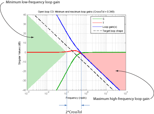
Where L is much greater than 1, a minimum gain constraint on
inv(S) (green shaded region) is equivalent to a minimum gain constraint on
L. Similarly, where L is much smaller than 1, a maximum
gain constraint on T (red shaded region) is equivalent to a maximum gain
constraint on L. The gap between these two constraints is twice the
CrossTol parameter, which specifies the frequency band where the loop gain
can cross 0 dB.
For multi-input, multi-output (MIMO) control systems, values in the gain profile greater
than 1 are interpreted as minimum performance requirements. Such values are lower bounds on the
smallest singular value of the open-loop response. Gain profile values less than one are
interpreted as minimum roll-off requirements, which are upper bounds on the largest singular
value of the open-loop response. For more information about singular values, see sigma.
Use TuningGoal.LoopShape when the loop shape near
crossover is simple or well understood (such as integral action). To specify only high gain or
low gain constraints in certain frequency bands, use TuningGoal.MinLoopGain and TuningGoal.MaxLoopGain. When you do so, the software
determines the best loop shape near crossover.
Creation
Syntax
Description
Req =
TuningGoal.LoopShape(location,loopgain)loopgain specifies the target open-loop gain profile. You can specify
the target gain profile (maximum gain across the I/O pair) as a smooth transfer function or
sketch a piecewise error profile using an frd model.
Req = TuningGoal.LoopShape(location,loopgain,crosstol)crosstol expresses the tolerance in decades. For example,
crosstol = 0.5 allows gain crossovers within half a decade on either
side of the target crossover frequency specified by loopgain. When you
omit crosstol, the tuning goal uses a default value of 0.1 decades. You
can increase crosstol when tuning MIMO control systems. Doing so allows
more widely varying crossover frequencies for different loops in the system.
Req = TuningGoal.LoopShape(
specifies a range for the target gain crossover frequency. The range is a vector of the form
location,wcrange)wcrange = [wc1,wc2]. This syntax is equivalent to
using the geometric mean sqrt(wc1*wc2) as wc and
setting crosstol to the half-width of wcrange in
decades. Using a range instead of a single wc value increases the ability
of the tuning algorithm to enforce the target loop shape for all loops in a MIMO control
system.
Input Arguments
Properties
Examples
Loop Shape and Crossover Tolerance
Create a target gain profile requirement for the following control system. Specify integral action, gain crossover at 1, and a roll-off requirement of 40 dB/decade.

The requirement should apply to the open-loop response measured at the AnalysisPoint block X. Specify a crossover tolerance of 0.5 decades.
LS = frd([100 1 0.0001],[0.01 1 100]);
Req = TuningGoal.LoopShape('X',LS,0.5);
The software converts LS into a smooth function of frequency that approximates the piecewise-specified requirement. Display the requirement using viewGoal.
viewGoal(Req)
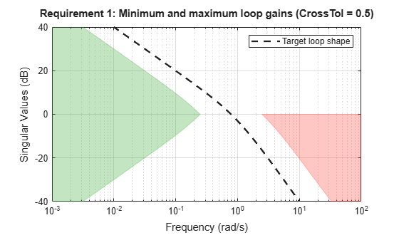
The green and red regions indicate the bounds for the inverse sensitivity, inv(S) = 1-G*C, and the complementary sensitivity, T = 1-S, respectively. The gap between these regions at 0 dB gain reflects the specified crossover tolerance, which is half a decade to either side of the target loop crossover.
When you use viewGoal(Req,CL) to validate a tuned closed-loop model of this control system, CL, the tuned values of S and T are also plotted.
Specify Different Loop Shapes for Multiple Loops
Create separate loop shape requirements for the inner and outer loops of the following control system.
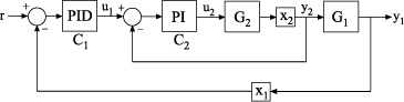
For the inner loop, specify a loop shape with integral action, gain crossover at 1, and a roll-off requirement of 40 dB/decade. Additionally, specify that this loop shape requirement should be enforced with the outer loop open.
LS2 = frd([100 1 0.0001],[0.01 1 100]);
Req2 = TuningGoal.LoopShape('X2',LS2);
Req2.Openings = 'X1';
Specifying 'X2' for the location indicates that Req2 applies to the point-to point, open-loop transfer function at the location X2. Setting Req2.Openings indicates that the loop is opened at the analysis point X1 when Req2 is enforced.
By default, Req2 imposes a stability requirement on the inner loop as well as the loop shape requirement. In some control systems, however, inner-loop stability might not be required, or might be impossible to achieve. In that case, remove the stability requirement from Req2 as follows.
Req2.Stabilize = false;
For the outer loop, specify a loop shape with integral action, gain crossover at 0.1, and a roll-off requirement of 20 dB/decade.
LS1 = frd([10 1 0.01],[0.01 0.1 10]);
Req1 = TuningGoal.LoopShape('X1',LS1);
Specifying 'X1' for the location indicates that Req1 applies to the point-to point, open-loop transfer function at the location X1. You do not have to set Req1.Openings because this loop shape is enforced with the inner loop closed.
You might want to tune the control system with both loop shaping requirements Req1 and Req2. To do so, use both requirements as inputs to the tuning command. For example, suppose CL0 is a tunable genss model of the closed-loop control system. In that case, use [CL,fSoft] = systune(CL0,[Req1,Req2]) to tune the control system to both requirements.
Loop Shape for Tuning Simulink Model
Create a loop-shape requirement for the feedback loop on 'q' in the Simulink model rct_airframe2. Specify that the loop-shape requirement is enforced with the 'az' loop open.
Open the model.
open_system('rct_airframe2')
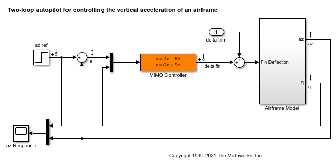
Create a loop shape requirement that enforces integral action with a crossover a 2 rad/s for the 'q' loop. This loop shape corresponds to a loop shape of 2/_s_.
s = tf('s');
shape = 2/s;
Req = TuningGoal.LoopShape('q',shape);
Specify the location at which to open an additional loop when enforcing the requirement.
Req.Openings = 'az';
To use this requirement to tune the Simulink model, create an slTuner interface to the model. Identify the block to tune in the interface.
ST0 = slTuner('rct_airframe2','MIMO Controller');
Designate both az and q as analysis points in the slTuner interface.
addPoint(ST0,{'az','q'});
This command makes q available as an analysis location. It also allows the tuning requirement to be enforced with the loop open at az.
You can now tune the model using Req and any other tuning requirements. For example:
[ST,fSoft] = systune(ST0,Req);
Final: Soft = 0.845, Hard = -Inf, Iterations = 51
Loop Shape Requirement with Crossover Range
Create a tuning requirement specifying that the open-loop response of loop identified by 'X' cross unity gain between 50 and 100 rad/s.
Req = TuningGoal.LoopShape('X',[50,100]);Examine the resulting requirement to see the target loop shape.
viewGoal(Req)

The plot shows that the requirement specifies an integral loop shape, with crossover around 70 rad/s, the geometrical mean of the range [50,100]. The gap at 0 dB between the minimum low-frequency gain (green region) and the maximum high-frequency gain (red region) reflects the allowed crossover range [50,100].
Tips
This tuning goal imposes an implicit stability constraint on the closed-loop sensitivity function measured at
Location, evaluated with loops opened at the points identified inOpenings. The dynamics affected by this implicit constraint are the stabilized dynamics for this tuning goal. TheMinDecayandMaxRadiusoptions ofsystuneOptionscontrol the bounds on these implicitly constrained dynamics. If the optimization fails to meet the default bounds, or if the default bounds conflict with other requirements, usesystuneOptionsto change these defaults.
Algorithms
When you tune a control system using a TuningGoal, the software converts
the tuning goal into a normalized scalar value f(x), where
x is the vector of free (tunable) parameters in the control system. The
software then adjusts the parameter values to minimize f(x)
or to drive f(x) below 1 if the tuning goal is a hard
constraint.
For TuningGoal.LoopShape, f(x) is
given by:
Here,
S = D–1[I – L(s,x)]–1D
is the scaled sensitivity function at the specified location, where
L(s,x) is the open-loop response being
shaped. D is an automatically-computed loop scaling factor. (If the
LoopScaling property is set to 'off', then
D = I.)
T = S – I is the
complementary sensitivity function.
WS and
WT are frequency weighting functions derived from the
specified loop shape. The gains of these functions roughly match LoopGain and
1/LoopGain, for values ranging from –20 dB to 60 dB. For numerical reasons,
the weighting functions level off outside this range, unless the specified loop gain profile
changes slope for gains above 60 dB or below –60 dB. Because poles of
WS or WT
close to s = 0 or s = Inf might lead to
poor numeric conditioning of the systune optimization problem, it is not
recommended to specify loop shapes with very low-frequency or very high-frequency
dynamics.
To obtain WS and WT, use:
[WS,WT] = getWeights(Req,Ts)
where Req is the tuning goal, and Ts is the sample
time at which you are tuning (Ts = 0 for continuous time). For more
information about the effects of the weighting functions on numeric stability, see Visualize Tuning Goals.
Version History
Introduced in R2016aSee Also
looptune | systune | looptune (for slTuner) (Simulink Control Design) | systune (for slTuner) (Simulink Control Design) | TuningGoal.MinLoopGain | TuningGoal.MaxLoopGain | viewGoal | TuningGoal.Tracking | TuningGoal.Gain | slTuner (Simulink Control Design) | frd
You can also select a web site from the following list:
Americas
- América Latina (Español)
- Canada (English)
- United States (English)
Europe
- Belgium (English)
- Denmark (English)
- Deutschland (Deutsch)
- España (Español)
- Finland (English)
- France (Français)
- Ireland (English)
- Italia (Italiano)
- Luxembourg (English)
- Netherlands (English)
- Norway (English)
- Österreich (Deutsch)
- Portugal (English)
- Sweden (English)
- Switzerland
- United Kingdom (English)