Analyze and Compress 1-D Convolutional Neural Network
This example shows how to analyze and compress a 1-D convolutional neural network used to estimate the frequency of complex-valued waveforms.
The network used in this example is a sequence-to-one regression network using the Complex Waveform data set, which contains 500 synthetically generated complex-valued waveforms of varying lengths with two channels. The network predicts the frequency of the waveforms.
The network in this example takes up about 45 KB of memory. If you want to use this model for inference, but have a memory restriction such as a limited-resource hardware target on which to embed the model, then you can compress the model. This example shows how to use Taylor pruning and projection to compress the network. You can use the same techniques to compress much larger networks.
For more information on how to train the 1-D convolutional neural network used in this example, see Train Network with Complex-Valued Data.
Load and Explore Network and Data
Load the network, training data, validation data, and test data.
load("ComplexValuedSequenceDataAndNetwork.mat")Compare the frequencies predicted by the pretrained network to the true frequencies for the first few sample sequences from the test set.
TPred = minibatchpredict(net,XTest, ...
    SequencePaddingDirection="left", ...
    InputDataFormats="CTB");

numChannels = 2;
displayLabels = [ ...
    "Real Part" + newline + "Channel " + string(1:numChannels), ...
    "Imaginary Part" + newline + "Channel " + string(1:numChannels)];

figure
tiledlayout(2,2)
for i = 1:4
nexttile

    stackedplot([real(XTest{i}') imag(XTest{i}')], DisplayLabels=displayLabels);

    xlabel("Time Step")
    title(["Predicted Frequency: " + TPred(i);"True Frequency: " + TTest(i)])
end

Calculate the root mean squared error of the network on the test data using the testnet function. Later, you use this value to verify that the compressed network is as accurate as the original network.
rmseOriginalNetwork = testnet(net,XTest,TTest,"rmse",InputDataFormats="CTB")
rmseOriginalNetwork =
0.8072
Analyze Network for Compression
Open the network in Deep Network Designer.
>> deepNetworkDesigner(net)
Get a report on how much compression pruning or projection of the network can achieve by clicking the Analyze for Compression button in the toolstrip.

The analysis report shows that you can compress the network using either pruning, projection, or quantization. You can also use a combination of more than one technique. If you combine pruning and projection, then prune before projecting.
Compress Network Using Pruning
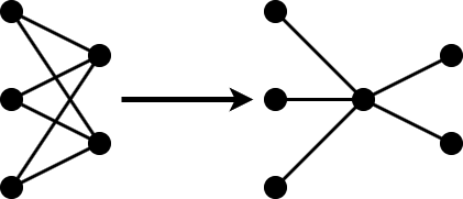
The compressNetworkUsingTaylorPruning function prunes a network iteratively using these steps:
Compute the importance score of each prunable filter.
Prune the least important filters.
Fine-tune the pruned network.
Specify Fine-Tuning Options
First, specify the training options for the fine-tuning step.
Specify the training options for the fine-tuning step. Use the same options that were used to train the original network, but use fewer training epochs. The network does not need to be trained from scratch, so you need fewer training epochs to retrain it.
The compressNetworkUsingTaylorPruning function applies the MaxEpochs training option to each fine-tuning period, during each pruning iteration. For example, if you set the LearnablesIncrement option to 0.05, then each pruning iteration removes approximately 5% of the original number of learnable parameters. In this case, pruning can comprise up to 20 pruning iterations, and the total number of training epochs can be as many as 20*MaxEpochs. Choosing the number of fine-tuning epochs is a tradeoff between pruning time and network accuracy.
In this example:
Train for 20 epochs using the Adam optimizer.
Set the learning rate schedule to
"piecewise".Specify the validation data.
To prevent overfitting, set
L2Regularizationto0.1.Set the
InputDataFormatsto"CTB"because the training data contains features in the first dimension, time-series sequences in the second dimension, and the batches of the data in the third dimension.Return the network with the best validation loss.
options = trainingOptions("adam", ...
    InputDataFormats="CTB", ...
    MaxEpochs=20, ...
    L2Regularization=0.1, ...
    ValidationData={XValidation, TValidation}, ...
    OutputNetwork="best-validation-loss");
Prune Pretrained Network
Compress the network using the compressNetworkUsingTaylorPruning function. To match the training configuration, specify the loss function as "mse" and specify the training options as options. Specify the learnables reduction goal as 0.6.
[netPruned,info] = compressNetworkUsingTaylorPruning(net,XTrain,TTrain,"mse",options,LearnablesReductionGoal=0.6);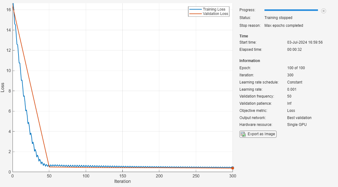
Compressed network has 60.4% fewer learnable parameters.
Pruning compressed 5 layers: "conv1d_1","layernorm_1","conv1d_2","layernorm_2","fc"
The pruning progress plot shows that in this example, the function performs 11 pruning iterations. During each iteration, the software tries to remove 5% of learnable parameters, until it exceeds the target learnables reduction. At the beginning of each pruning iteration, the loss spikes, but then recovers during fine-tuning.
Test the pruned network. Compare the RMSE of the pruned and original networks.
rmsePrunedNetwork = testnet(netPruned,XTest,TTest,"rmse",InputDataFormats="CTB")
rmsePrunedNetwork =
0.7807
rmseOriginalNetwork
rmseOriginalNetwork =
0.8072
The RMSE of the pruned network is similar to the RMSE of the original network. If your network loses accuracy due to the pruning process, you can retrain the network for several epochs to regain some of the lost accuracy.
Compress Network Using Projection
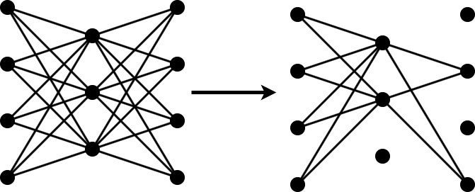
Projection allows you to convert large layers with many learnables to one or more smaller layers with fewer learnable parameters in total.
The compressNetworkUsingProjection function applies principal component analysis (PCA) to the training data to identify the subspace of learnable parameters that result in the highest variance in neuron activations.
First, reanalyze the pruned network for compression using Deep Network Designer.

The analysis report shows that you can further compress the network using both pruning and projection.
Project the network using the compressNetworkUsingProjection function. Specify a learnables reduction goal of 70%.
[netProjected,info] = compressNetworkUsingProjection(netPruned,XTrain,InputDataFormats="CTB",LearnablesReductionGoal=0.7);Compressed network has 70.4% fewer learnable parameters. Projection compressed 2 layers: "conv1d_1","conv1d_2"
Test the projected network. Compare the RMSE of the projected and original networks.
testnet(netProjected,XTest,TTest,"rmse",InputDataFormats="CTB")
ans =
1.2561
rmseOriginalNetwork
rmseOriginalNetwork =
0.8072
Retrain Projected Network
Use the trainnet function to retrain the network for several epochs and regain some of the lost accuracy. Increase the maxEpochs training option to 200.
options.MaxEpochs = 200;
netProjected = trainnet(XTrain,TTrain,netProjected,"mse",options);
Iteration Epoch TimeElapsed LearnRate TrainingLoss ValidationLoss
_________ _____ ___________ _________ ____________ ______________
0 0 00:00:00 0.001 1.3861
1 1 00:00:00 0.001 1.4418
50 17 00:00:03 0.001 0.60451 0.65735
100 34 00:00:05 0.001 0.51409 0.60985
150 50 00:00:06 0.001 0.48094 0.58628
200 67 00:00:07 0.001 0.50838 0.57827
250 84 00:00:08 0.001 0.44913 0.56529
300 100 00:00:09 0.001 0.41447 0.54827
350 117 00:00:11 0.001 0.46785 0.53551
400 134 00:00:12 0.001 0.41301 0.52036
450 150 00:00:14 0.001 0.39008 0.52136
500 167 00:00:15 0.001 0.43596 0.5382
550 184 00:00:16 0.001 0.38335 0.51914
600 200 00:00:17 0.001 0.37476 0.5131
Training stopped: Max epochs completed
Test the fine-tuned projected network. Compare the RMSE of the fine-tuned projected and original networks.
rmseProjectedNetwork = testnet(netProjected,XTest,TTest,"rmse",InputDataFormats="CTB")
rmseProjectedNetwork =
0.8245
rmseOriginalNetwork
rmseOriginalNetwork =
0.8072
Compare Networks
Compare the size and accuracy of the original network, the fine-tuned pruned network, and the fine-tuned pruned and projected network.
infoOriginalNetwork = analyzeNetwork(net,Plots="none");
infoPrunedNetwork = analyzeNetwork(netPruned,Plots="none");
infoProjectedNetwork = analyzeNetwork(netProjected,Plots="none");

numLearnablesOriginalNetwork = infoOriginalNetwork.TotalLearnables;
numLearnablesPrunedNetwork = infoPrunedNetwork.TotalLearnables;
numLearnablesProjectedNetwork = infoProjectedNetwork.TotalLearnables;

figure
tiledlayout("flow")

nexttile
bar([rmseOriginalNetwork rmsePrunedNetwork rmseProjectedNetwork])
xticklabels(["Original" "Pruned" "Pruned and Projected"])
title("RMSE")
ylabel("RMSE")

nexttile
bar([numLearnablesOriginalNetwork numLearnablesPrunedNetwork numLearnablesProjectedNetwork])
xticklabels(["Original" "Pruned" "Pruned and Projected"])
ylabel("Number of Learnables")
title("Number of Learnables")

The plot compares the RMSE as well as the number of learnable parameters of the original network, the fine-tuned pruned network, and the fine-tuned pruned and projected network. The number of learnables decreases significantly with each compression step, without any negative impact on the RMSE.