Liquid Hydrogen Storage and Transportation
This example shows how to model a cryogenic tank by using Simscape™ Fluids™ blocks. Aviation and aerospace applications commonly use liquid hydrogen storage instead of compressed gas storage. Engineering challenges include minimizing liquid boil-off, managing tank internal pressure, and designing a robust storage tank.
Liquid hydrogen is stored at approximately 20 K. Tank pressure can increase due to liquid boil-off, caused by heat ingress, hydrogen isomer reaction, and slosh energy during tank transport. To mitigate boil-off, the tank typically has three layers: a low thermal conductivity inner layer, a vacuum layer, and a low thermal conductivity outer layer. Hydrogen embrittlement at low temperatures influences the material choice and thickness, which contribute to the tank weight and energy density. This example demonstrates verifying the tank mechanical design against the hydrogen boil-off and tank pressure increase.
Define System
![]()
This example simulates tank fill, tank transportation, and tank storage at rest. The image shows the cryogenic tank with an inlet port, a liquid outlet port, and a gas vent. A pump fills the hydrogen from a reservoir. During filling, the liquid outlet and vent are closed. As pressure rises, the vent opens to release gas and maintain a specified pressure within the tank. The Two-Phase Fluid Properties (2P) block is parameterized with hydrogen properties by using the twoPhaseFluidTables function.
Initialize the system model:
open_system("LiquidHydrogenStorageAndTransportation")
run("LiquidHydrogenStorageAndTransportationParameters")
Specify Requirements
The tank is filled and transported in the span of a few hours. The process is as follows:
Filling starts when the tank is nearly empty; the fill liquid ortho-isomer ratio is
0.1.Tank fill time is
20 min.Road transportation time is
1.5 hr.Then, the tank is at rest for
22 hr.
The key design requirements are:
The pressure inside the tank must remain below 1 MPa.
Maximum boil-off rate must be less than 1% mass per day.
SysParams.PressureMax    = 1;     % Maximum tank pressure, MPa
SysParams.MaxBoilOffRate = 1/100; % Maximum boil-off rate
Specify Tank Geometry
This example uses a cylindrical tank. Specify the tank geometry:
InputParam.TankLen = 4.15; % Tank length, m
InputParam.TankDia = 1.6;  % Tank diameter, m
InputParam.PipeDia = 0.11; % Diameter of pipe connections, m
Update model parameters based on user-defined inputs:
Tank.CrossSectionalArea = 0.25*pi*InputParam.TankDia^2;
Tank.Volume = Tank.CrossSectionalArea*InputParam.TankLen;
![]()
The tank is modeled using the Receiver Accumulator (2P) block in Simscape Fluids. The liquid and vapor occupy separate volumes inside the block. Some liquid warms as it evaporates and transfers to the vapor volume. The lower vapor density increases the tank pressure, requiring periodic venting to remain below maximum pressure. This is the boil-off loss.
Model Boil-off Losses
![]()
The thermal network connected to port H of the Receiver Accumulator (2P) block models the hydrogen physics related to boil-off. The Boil-Off Model subsystem contains three subsystems that model:
Slosh
Ambient heat transfer, and
Hydrogen isomer conversion
Model Heat Exchange with Environment
The impact of environment is modeled using thermal networks for heat conduction, convection, and radiation. The three layers of the tank wall are modeled as the inner wall, the outer wall, and the insulation layer. The tank outer wall gains energy from the environment through convective and radiative heat transfer.
Specify the tank outer vessel properties:
Tank.OuterWall.Thickness = 3e-2; % Thickness, meters
Tank.OuterWall.ThermalK = 5e-2;  % Thermal conductivity, W/m*K
Tank.OuterWall.Density = 2400;   % Material density, kg/cu.m
Tank.OuterWall.SpHeat = 800;     % Heat Capacity, J/kg.K
Specify the tank insulation layer properties:
Tank.Insulation.Thickness = 5e-3; % Thickness, meters
Tank.Insulation.ThermalK = 1e-4;  % Thermal conductivity, W/m*K
Tank.Insulation.Density = 1.25;   % Material density, kg/cu.m
Tank.Insulation.SpHeat = 1;       % Heat Capacity, J/kg.K
Specify the tank inner vessel properties:
Tank.InnerWall.Thickness = 2e-2; % Thickness, meters
Tank.InnerWall.ThermalK = 5e-2;  % Thermal conductivity, W/m*K
Tank.InnerWall.Density = 800;    % Material density, kg/cu.m
Tank.InnerWall.SpHeat = 400;     % Heat Capacity, J/kg.K
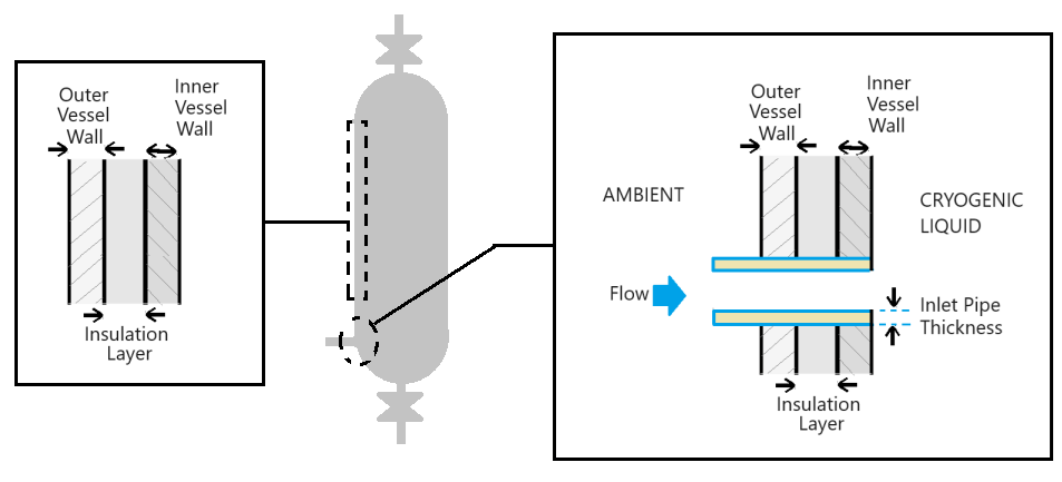
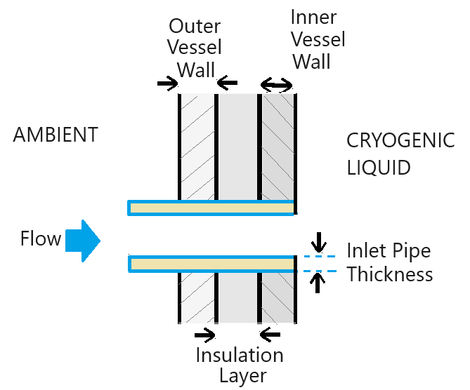
The tank has two pipe connections for the liquid pipe and the vapor vent pipe. The liquid filling line and liquid withdrawal line in the tank both connect to the liquid pipe. The safety vent line connects to the vapor vent pipe. The pipes are typically not as well insulated and present a heat transfer path into the tank. The schematic shows the heat transfer model:
Specify the vapor vent pipe parameters:
Tank.VentPipe.Area = 0.25*pi*InputParam.PipeDia^2; % Tank pressure vent cross-sectional area, m^2
Tank.VentPipe.Thickness = 0.006;                   % Vent pipe thickness, m
Tank.VentPipe.Length = 0.1;                        % Vent pipe length, m
Tank.VentPipe.ThermalK = 5;                        % Vent pipe thermal conductivity, W/m*K
Specify the liquid tapping pipe parameters:
Tank.LiqPipe.Area = 0.25*pi*InputParam.PipeDia^2; % Tank liquid tapping point cross-sectional area, m^2
Tank.LiqPipe.Thickness = 0.006;                   % Liquid tapping pipe thickness, m
Tank.LiqPipe.Length = 0.1;                        % Liquid tapping pipe length, m
Tank.LiqPipe.ThermalK = 5;                        % Liquid tapping pipe thermal conductivity, W/m*K
The tank wall model has three layers:
The inner vessel in contact with hydrogen
The insulating or vacuum layer, and
The outer vessel in contact with the environment.
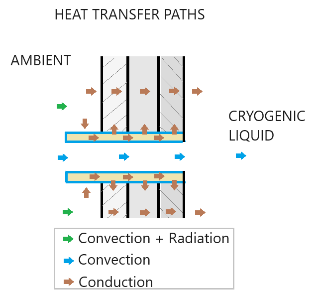
The pipes conduct heat to the three tank wall layers. The subsystem SegmentedPipeFittings models the three pipes, each of which is segmented based on the tank wall thickness. The pipe metal conducts heat into the tank and to the tank vessel, as represented in the block diagram.
![]()
Model Isomer Conversion Heat Generation
Hydrogen has two isomers: ortho and para. At room temperature, hydrogen composition is 75% ortho and 25% para isomer. The two isomers have slightly different thermal properties, but almost the same chemical properties. At temperatures as low as 20 K, liquid hydrogen exists predominantly as para isomer. Ortho-hydrogen conversion to para-hydrogen releases energy. Para-hydrogen conversion to ortho-hydrogen absorbs energy.
Uncatalyzed conversion of ortho-hydrogen to para-hydrogen happens slowly. During liquefaction, incomplete conversion can release during storage from the ortho-hydrogen converting to para equilibrium at low temperatures. Different components may have different isomer ratio and the flow of fluid through tanks, storage, pipes can lead to isomer heat generation. A custom component models the isomer conversion heat generation.
![]()
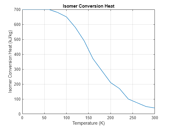
Specify the ortho-isomer fraction for the liquid in the tank and for the liquid flowing into the tank separately. The plot shows the specific enthalpy of isomer conversion versus temperature:
figure
plot(Hydrogen.TempVec, Hydrogen.EnthalpyVec, LineWidth = 1)
grid on
xlabel("Temperature (K)")
ylabel("Isomer Conversion Heat (kJ/kg)")
title("Isomer Conversion Heat")
The rate of isomer conversion is modeled using first-order dynamics based on the reaction rate constant . Doing a mass balance of ortho-hydrogen in the tank gives differential equation for the ortho-hydrogen fraction in the tank:
where
, , and are, respectively, the mass fractions of ortho-hydrogen in the tank, at equilibrium, and for inflow during filling
is the liquid mass in the tank
is the liquid mass flow rate into the tank during filling
The rate of heat generated by the conversion is:
where is the specific enthalpy of the isomer conversion as a function of the liquid temperature. The Simscape language file LiquidHydrogenIsomerConversion.ssc implements the equations for the custom component.
Model Impact of Slosh
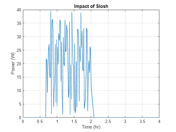
The liquid slosh during transportation increases the kinetic energy of fluid and fluid mixing. This increase leads to a more uniform temperature in the fluid, changes in heat transfer, and heat generation due to the fluid impact on walls. The vehicle transporting the tank moves between t = 30 min and t = 2 hr. After 2 hours, the tank is at rest. This example assumes that the rate of heat addition due to slosh can be derived from experimental measurements:
load LiquidHydrogenSloshImpact.mat
figure
plot(SloshImpact.Time/3600, squeeze(SloshImpact.Data), LineWidth = 1)
grid on
xlabel("Time (hr)")
ylabel("Power (W)")
title("Impact of Slosh")
Evaluate Design
Set the average temperature during the day:
SysParams.AmbientT = 300;   % Ambient temperature, K
SysParams.AmbientTvar = 10; % Ambient temperature variation amplitude during the day, K
Set the tank fill time:
SysParams.TankFillTime = 1200; % Time for which tank is filled, s
SysParams.TankFillRate = 0.4;  % Tank fill rate, kg/s
Set the initial ortho-isomer fraction in the tank:
Hydrogen.OrthoInit = 0.1; % Initial ortho-isomer mass fraction in tank (post liquefaction)Set the ortho-isomer fraction in the incoming liquid flow:
Hydrogen.OrthoInflow = 0.13; % Ortho-isomer mass fraction in incoming flow (post liquefaction)Enable slosh modeling:
SysParams.SloshModelOpt = 1; % Set 1/0 to model/not-model slosh impactWhen flow through a two-phase fluid node changes direction, the internal energy advected through the node changes between the former and new upstream values. The internal energy change is smoothed for numerical robustness. Smoothing the internal energy change manifests as a slight heat transfer through the node, analogous to conduction.
Because of the very low heat transfer rate of the boil-off energy loss, modeling cannot neglect the additional heat transfer effect due to numerical smoothing. Therefore, the smoothing parameter value in the Two-Phase Fluid Properties (2P) block reduces from 0.01 (default) to 1e-4:
SysParams.SmoothRevThres = 1e-4; % Dynamic pressure threshold for smoothed flow reversal, PaRun the simulation for tank filling, transport (1.5 hr), and storage (approximately 22 hr) for a full day:
simResult = sim("LiquidHydrogenStorageAndTransportation", "StopTime", "3600*24");
data = simResult.logsout.extractTimetable;
time = hours(data.Time);
time_s = seconds(data.Time);
Plot Results
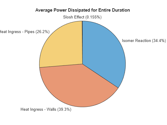
Plot the heat ingress due to individual sources:
result.totalTime = time_s(end) - time_s(1);
result.heatGenMech = ["Isomer Reaction"; "Heat Ingress - Walls"; "Heat Ingress - Pipes"; "Slosh Effect"];
result.avgPow = [
    trapz(time_s, data.("Heat.isomer"));
    trapz(time_s, data.("Heat.vesselWalls"));
    trapz(time_s, data.("Heat.pipeFittings"));
    trapz(time_s, data.("Heat.slosh"))] / result.totalTime;
result.avgPowPercent = round(result.avgPow*100/sum(result.avgPow), 1);
result.avgPowPlot = table(result.heatGenMech, result.avgPow, result.avgPowPercent);
result.avgPowPlot.Properties.VariableNames = ["Mechanism", "Power Added (W)", "% Contribution"];
figure
piechart(result.avgPow, result.heatGenMech)
title("Average Power Dissipated for Entire Duration")
Display the data for heat ingress due to individual sources:
disp(result.avgPowPlot)
          Mechanism           Power Added (W)    % Contribution
    ______________________    _______________    ______________

    "Isomer Reaction"             256.31              34.4
    "Heat Ingress - Walls"        293.05              39.3
    "Heat Ingress - Pipes"        194.99              26.2
    "Slosh Effect"                1.1539               0.2
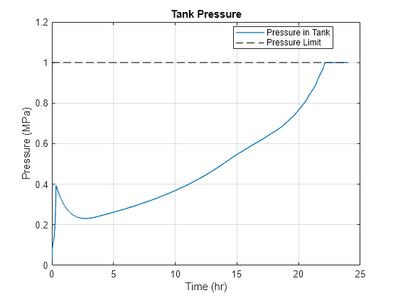
Plot the tank pressure change vs. time:
figure
plot(time, data.("pressure"), LineWidth = 1)
hold on
plot([time(1) time(end)], [1 1]*SysParams.PressureMax, "k--")
hold off
grid on
xlabel("Time (hr)")
ylabel("Pressure (MPa)")
title("Tank Pressure")
legend("Pressure in Tank", "Pressure Limit", Location = "best")
Calculate the boil-off rate by integrating the gas outflow rate to obtain the mass lost and integrating the liquid inflow rate to obtain the mass supplied:
result.boilOffRate = trapz(time_s, data.("Outflow.g")) ...
    / (data.("mass")(1) + trapz(time_s, data.("inflow")));
if result.boilOffRate > SysParams.MaxBoilOffRate
    result.dispMessage = "Tank boil-off rate (" + result.boilOffRate*100 + " percent per day) does not meet the requirements (" + SysParams.MaxBoilOffRate*100 + " percent per day)";
else
    result.dispMessage = "Tank boil-off rate (" + result.boilOffRate*100 + " percent per day) meets the requirements (" + SysParams.MaxBoilOffRate*100 + " percent per day)";
end
disp(result.dispMessage)
Tank boil-off rate (0.99327 percent per day) meets the requirements (1 percent per day)
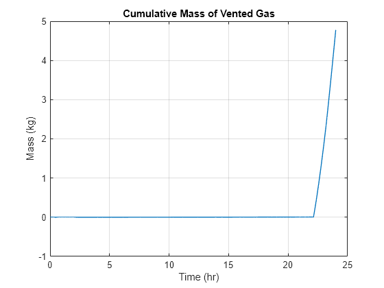
Plot the amount of vented hydrogen gas:
figure
plot(time, cumtrapz(time_s, data.("Outflow.g")), LineWidth = 1)
grid on
xlabel("Time (hr)")
ylabel("Mass (kg)")
title("Cumulative Mass of Vented Gas")
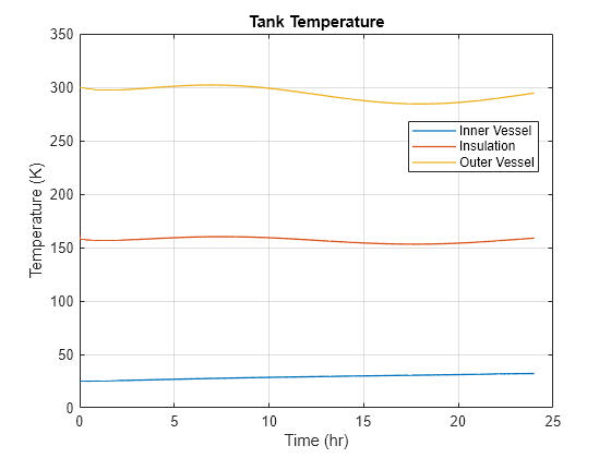
Plot the tank surface temperature:
figure
plot(time, data.("TankTemp.innerVessel"), LineWidth = 1)
hold on
plot(time, data.("TankTemp.insulation"), LineWidth = 1)
plot(time, data.("TankTemp.outerVessel"), LineWidth = 1)
hold off
grid on
xlabel("Time (hr)")
ylabel("Temperature (K)")
title("Tank Temperature")
legend("Inner Vessel", "Insulation", "Outer Vessel", Location = "best")
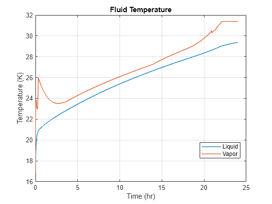
Plot the fluid temperature inside the tank:
figure
plot(time, data.("H2Temp.liq"), LineWidth = 1)
hold on
plot(time, data.("H2Temp.vap"), LineWidth = 1)
hold off
grid on
xlabel("Time (hr)")
ylabel("Temperature (K)")
title("Fluid Temperature")
legend("Liquid", "Vapor", Location = "best")