Estimate MIMO State-Space Model Using AAA Algorithm

R2026b

This example demonstrates how to identify a state-space model to fit a multi-input multi-output (MIMO) frequency response using the Adaptive Antoulas-Anderson (AAA) algorithm within the ssest function. The example also estimates a state-space model using the traditional N4SID algorithm and shows that the AAA algorithm is not only faster but also provides a better fit score.

Data Preparation

Load a non-uniformly sampled frequency domain data set with four inputs and four outputs.

load frd44.mat frddata

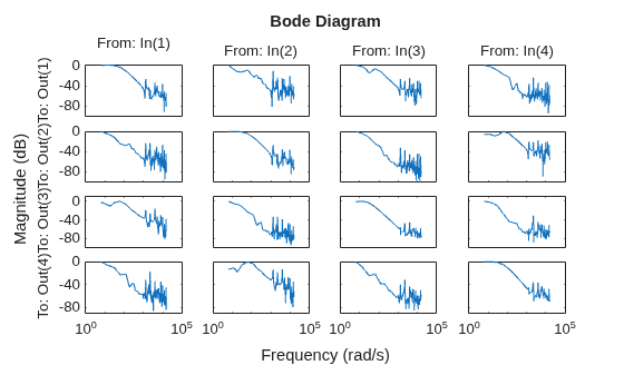
Visualize the response magnitude using the bodemag command.

bodemag(frddata)

Model Estimation Using AAA Algorithm

To initialize the state-space parameters using the AAA algorithm, specify the InitializeMethod property of the ssestOptions option set as 'AAA'. To disable the nonlinear optimization that occurs after the AAA algorithm stops and to display the results obtained only from the AAA algorithm, set the MaxIterations property to be 0. Optionally, you can enable further fine-tuning of the results by setting the MaxIterations property to a positive integer.

opt_aaa = ssestOptions;
opt_aaa.InitializeMethod = "AAA";
opt_aaa.SearchOptions.MaxIterations = 0;
opt_aaa.EstimateCovariance = false;

Specify the AAA error tolerance as 1e-2. For MIMO systems, in each iteration, the AAA algorithm adds a real pole or a pair of complex-conjugate poles until the fitting error is below this tolerance or the limit on the number of unique poles is reached. For more information on the AAA algorithm and the error tolerance, see the InitializeMethod property and the AAATolerance option under the Advanced property of the ssestOptions object.

opt_aaa.Advanced.AAATolerance = 1e-2;

Specify the maximum number of unique poles allowed in the model, nx. If you specify nx as "best", the algorithm automatically determines the optimal value of nx. For more information, see the nx input argument in ssest.

nx = "best";

The model has more parameters than data samples, which causes a warning. Suppress this warning before calling ssest.

Warn = warning('off','Ident:estimation:NparGTNsamp');
WarnReset = onCleanup(@()warning(Warn));

Estimate a discrete-time state-space model using ssest.

sys_aaa = ssest(frddata,nx,opt_aaa,Ts=frddata.Ts);

Model Estimation Using N4SID Algorithm

To initialize the state-space parameters using the N4SID algorithm, specify the InitializeMethod property of the ssestOptions option set as 'n4sid' and the MaxIterations property as false.

opt_n4sid = ssestOptions;
opt_n4sid.InitializeMethod = "n4sid";
opt_n4sid.SearchOptions.MaxIterations = 0;
opt_n4sid.EstimateCovariance = false;

Specify the model order to be same as that estimated using the AAA algorithm.

nx_n4sid = order(sys_aaa);

Estimate a discrete-time state-space model using ssest.

sys_n4sid = ssest(frddata,nx_n4sid,opt_n4sid,Ts=frddata.Ts);

Visualize the response magnitude.

bodemag(frddata,'k',sys_aaa,sys_n4sid)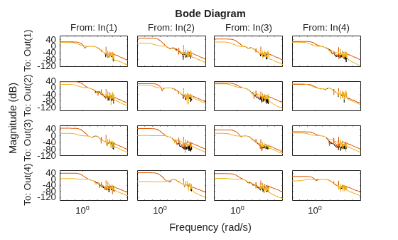

Model Refinement Using Numerical Search

You can improve the estimated models by using numerical search algorithms.

In this example, fine-tune the model sys_aaa using the Levenberg–Marquardt least squares search approach. For more information, see the SearchMethod property of ssestOptions.

opt_aaa.SearchMethod = "lm";
opt_aaa.SearchOptions.MaxIterations = 20;
opt_aaa.OutputWeight = eye(4);
sys_aaa_improved = ssest(frddata,sys_aaa,opt_aaa);

Comparison of Results

Calculate the fit percentages of all the estimated models.

fit_aaa = sys_aaa.Report.Fit.FitPercent

fit_aaa = 4×4

   94.9337   79.0105   90.6819   89.1039
   91.8608   95.0797   95.3417   89.4936
   90.2435   87.6078   98.0454   88.8057
   93.7053   90.1604   90.9233   95.5113

fit_n4sid = sys_n4sid.Report.Fit.FitPercent

fit_n4sid = 4×4

   91.1242   78.4726   87.6710   82.5904
   89.9686   91.5256   88.8637   87.3323
   91.3781   85.3370   92.9799   85.6339
   88.8730   83.2124   79.9640   90.9906

fit_aaa_improved = sys_aaa_improved.Report.Fit.FitPercent

fit_aaa_improved = 4×4

   98.6779   89.7592   97.1534   97.5046
   94.8708   98.7158   98.8727   92.2033
   95.7501   99.1115   99.6366   98.9381
   97.2711   92.6278   98.3328   98.9377

You can see that the AAA algorithm returns better results when compared to the N4SID algorithm.

Calculate and plot the improvement in the fit scores from the N4SID to the AAA algorithms.

fitImprove = fit_aaa - fit_n4sid;
heatmap(fitImprove, 'Title', 'Fit Score Improvements (fit_{aaa} - fit_{n4sid})')
xlabel('Inputs')
ylabel('Outputs')

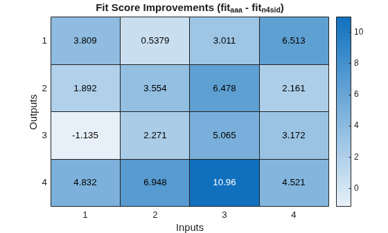
The AAA algorithm clearly outperforms the N4SID algorithm in all channels.

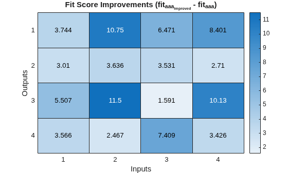
Similarly, analyze the improved model obtained by using the numerical search algorithm.

fitGain = fit_aaa_improved - fit_aaa;
heatmap(fitGain, 'Title', 'Fit Score Improvements (fit_{aaa_{improved}} - fit_{aaa})')
xlabel('Inputs')
ylabel('Outputs')

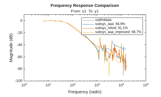
Compare the frequency responses of all the estimated state-space models against the measured frequency response data using the compare command. For example, compare the responses corresponding to the first input and output. You can verify the better performance of the AAA algorithm.

subfrddata = frddata(1,1);
subsys_aaa = sys_aaa(1,1);
subsys_n4sid = sys_n4sid(1,1);
subsys_aaa_improved = sys_aaa_improved(1,1);

figure
compare(subfrddata,subsys_aaa,subsys_n4sid,subsys_aaa_improved)
legend("show",Interpreter="none")