Quadratic Programming for Portfolio Optimization Problems, Solver-Based

R2026b

This example shows how to solve portfolio optimization problems using the interior-point quadratic programming algorithm in quadprog. The function quadprog belongs to Optimization Toolbox™.

The matrices that define the problems in this example are dense; however, the interior-point algorithm in quadprog can also exploit sparsity in the problem matrices for increased speed. For a sparse example, see Large Sparse Quadratic Program with Interior Point Algorithm.

The Quadratic Model

Suppose that there are $n$ different assets. The rate of return of asset $i$ is a random variable with expected value $m_{i}$ . The problem is to find what fraction $x_{i}$ to invest in each asset $i$ in order to minimize risk, subject to a specified minimum expected rate of return.

Let $C$ denote the covariance matrix of rates of asset returns.

The classical mean-variance model consists of minimizing portfolio risk, as measured by

$\frac{1}{2} x^{T} C x$

subject to a set of constraints.

The expected return should be no less than a minimal rate of portfolio return $r$ that the investor desires,

$\sum_{i = 1}^{n} m_{i} x_{i} \geq r,$

the sum of the investment fractions $x_{i}$ 's should add up to a total of one,

$\sum_{i = 1}^{n} x_{i} = 1,$

and, being fractions (or percentages), they should be numbers between zero and one,

$0 \leq x_{i} \leq 1, i = 1 \dots n .$

Since the objective to minimize portfolio risk is quadratic, and the constraints are linear, the resulting optimization problem is a quadratic program, or QP.

225-Asset Problem

Let us now solve the QP with 225 assets. The dataset is from the OR-Library [Chang, T.-J., Meade, N., Beasley, J.E. and Sharaiha, Y.M., "Heuristics for cardinality constrained portfolio optimisation" Computers & Operations Research 27 (2000) 1271-1302].

We load the dataset and then set up the constraints in a format expected by quadprog. In this dataset the rates of return $m_{i}$ range between –0.008489 and 0.003971; we pick a desired return $r$ in between, e.g., 0.002 (0.2 percent).

Load dataset stored in a MAT-file.

load("port5.mat","Correlation","stdDev_return","mean_return")

Calculate covariance matrix from correlation matrix.

Covariance = Correlation .* (stdDev_return * stdDev_return');
nAssets = numel(mean_return); r = 0.002;     % number of assets and desired return
Aeq = ones(1,nAssets); beq = 1;              % equality Aeq*x = beq
Aineq = -mean_return'; bineq = -r;           % inequality Aineq*x <= bineq
lb = zeros(nAssets,1); ub = ones(nAssets,1); % bounds lb <= x <= ub
c = zeros(nAssets,1);                        % objective has no linear term; set it to zero

Select the Interior Point Algorithm in Quadprog

In order to solve the QP using the interior-point algorithm, we set the option Algorithm to "interior-point-convex".

options = optimoptions("quadprog",Algorithm="interior-point-convex");

Solve 225-Asset Problem

We now set some additional options, and call the solver quadprog.

Set additional options: turn on iterative display, and set a tighter optimality termination tolerance.

options = optimoptions(options,Display="iter",TolFun=1e-10);

Call solver and measure wall-clock time.

tic
[x1,fval1] = quadprog(Covariance,c,Aineq,bineq,Aeq,beq,lb,ub,[],options);

 Iter            Fval  Primal Infeas    Dual Infeas  Complementarity   Wall-Clock Time  
    0    2.384401e+01   2.253410e+02   1.337381e+00     1.000000e+00      0.010899 sec  
    1    1.338822e-03   7.394864e-01   4.388791e-03     1.038098e-02      0.013597 sec  
    2    1.186079e-03   6.443975e-01   3.824446e-03     8.727381e-03      0.016201 sec  
    3    5.923977e-04   2.730703e-01   1.620650e-03     1.174211e-02      0.017235 sec  
    4    5.354880e-04   5.303581e-02   3.147632e-04     1.549549e-02      0.018875 sec  
    5    5.181994e-04   2.651791e-05   1.573816e-07     2.848171e-04      0.020082 sec  
    6    5.066191e-04   9.285375e-06   5.510794e-08     1.041224e-04      0.021072 sec  
    7    3.923090e-04   7.619855e-06   4.522322e-08     5.536006e-04      0.022048 sec  
    8    3.791545e-04   1.770065e-06   1.050519e-08     1.382075e-04      0.023050 sec  
    9    2.923749e-04   8.850312e-10   5.252599e-12     3.858983e-05      0.023977 sec  
   10    2.277722e-04   4.431702e-13   2.627914e-15     6.204101e-06      0.024911 sec  
   11    1.992243e-04   2.229120e-16   2.127959e-18     4.391483e-07      0.025887 sec  
   12    1.950468e-04   3.339343e-16   1.456847e-18     1.429441e-08      0.028161 sec  
   13    1.949141e-04   3.330669e-16   1.239159e-18     9.731942e-10      0.029922 sec  
   14    1.949121e-04   8.886121e-16   6.938894e-18     2.209702e-12      0.031055 sec  

Minimum found that satisfies the constraints.

Optimization completed because the objective function is non-decreasing in 
feasible directions, to within the value of the optimality tolerance,
and constraints are satisfied to within the value of the constraint tolerance.

<stopping criteria details>

toc

Elapsed time is 0.049400 seconds.

Plot results.

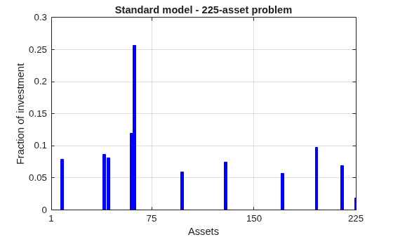
plotPortfDemoStandardModel(x1)

$Bar chart of optimal investment fractions for the 225-asset standard model, showing most weight concentrated in a few assets$

225-Asset Problem with Group Constraints

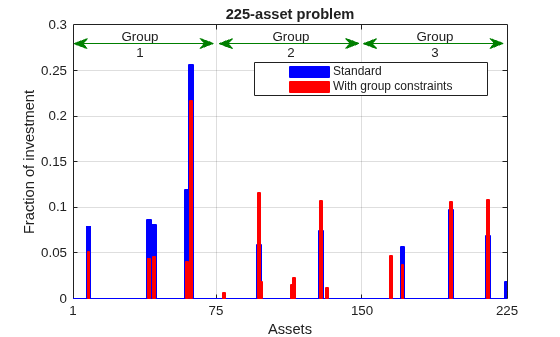
We now add to the model group constraints that require that 30% of the investor's money has to be invested in assets 1 to 75, 30% in assets 76 to 150, and 30% in assets 151 to 225. Each of these groups of assets could be, for instance, different industries such as technology, automotive, and pharmaceutical. The constraints that capture this new requirement are

$\sum_{i = 1}^{75} x_{i} \geq 0.3,$

$\sum_{i = 76}^{150} x_{i} \geq 0.3,$

$\sum_{i = 151}^{225} x_{i} \geq 0.3 .$

Add group constraints to existing equalities.

Groups = blkdiag(ones(1,nAssets/3),ones(1,nAssets/3),ones(1,nAssets/3));
Aineq = [Aineq; -Groups];         % convert to <= constraint
bineq = [bineq; -0.3*ones(3,1)];  % by changing signs

Call solver and measure wall-clock time.

tic
[x2,fval2] = quadprog(Covariance,c,Aineq,bineq,Aeq,beq,lb,ub,[],options);

 Iter            Fval  Primal Infeas    Dual Infeas  Complementarity   Wall-Clock Time  
    0    2.384401e+01   4.464410e+02   1.337324e+00     1.000000e+00      0.014846 sec  
    1    1.346872e-03   1.474737e+00   4.417606e-03     3.414918e-02      0.018766 sec  
    2    1.190113e-03   1.280566e+00   3.835962e-03     2.934585e-02      0.019984 sec  
    3    5.990845e-04   5.560762e-01   1.665738e-03     1.320038e-02      0.021216 sec  
    4    3.890097e-04   2.780381e-04   8.328691e-07     7.287370e-03      0.022435 sec  
    5    3.887354e-04   1.480950e-06   4.436215e-09     4.641988e-05      0.023652 sec  
    6    3.387787e-04   8.425389e-07   2.523843e-09     2.578178e-05      0.024865 sec  
    7    3.089240e-04   2.707587e-07   8.110632e-10     9.217509e-06      0.026066 sec  
    8    2.639458e-04   6.586817e-08   1.973095e-10     6.509001e-06      0.027276 sec  
    9    2.252657e-04   2.225507e-08   6.666551e-11     6.783212e-06      0.028496 sec  
   10    2.105838e-04   5.811527e-09   1.740855e-11     1.967570e-06      0.029699 sec  
   11    2.024362e-04   4.129834e-12   1.237133e-14     5.924109e-08      0.030909 sec  
   12    2.009704e-04   3.787335e-15   1.441446e-17     6.354389e-10      0.032113 sec  
   13    2.009650e-04   6.665675e-16   6.938894e-18     1.889136e-13      0.033325 sec  

Minimum found that satisfies the constraints.

Optimization completed because the objective function is non-decreasing in 
feasible directions, to within the value of the optimality tolerance,
and constraints are satisfied to within the value of the constraint tolerance.

<stopping criteria details>

toc

Elapsed time is 0.051104 seconds.

Plot results, superimposed on results from previous problem.

plotPortfDemoGroupModel(x1,x2);

Bar chart comparing standard and group-constrained portfolio allocations across 225 assets, showing more even distribution with group constraints

Summary of Results So Far

We see from the second bar plot that, as a result of the additional group constraints, the portfolio is now more evenly distributed across the three asset groups than the first portfolio. This imposed diversification also resulted in a slight increase in the risk, as measured by the objective function (see column labeled "f(x)" for the last iteration in the iterative display for both runs).

1000-Asset Problem Using Random Data

In order to show how quadprog's interior-point algorithm behaves on a larger problem, we'll use a 1000-asset randomly generated dataset. We generate a random correlation matrix (symmetric, positive-semidefinite, with ones on the diagonal) using the gallery function in MATLAB®.

Reset the random stream for reproducibility.

rng(0,"twister");
nAssets = 1000; % desired number of assets

Generate means of returns between –0.1 and 0.4.

a = -0.1; b = 0.4;
mean_return = a + (b-a).*rand(nAssets,1);

Generate standard deviations of returns between 0.08 and 0.6.

a = 0.08; b = 0.6;
stdDev_return = a + (b-a).*rand(nAssets,1);
% Correlation matrix, generated using Correlation = gallery("randcorr",nAssets).
% (Generating a correlation matrix of this size takes a while, so we load
% a pre-generated one instead.)
load("correlationMatrixDemo.mat","Correlation");
% Calculate covariance matrix from correlation matrix.
Covariance = Correlation .* (stdDev_return * stdDev_return');

Define and Solve Randomly Generated 1000-Asset Problem

We now define the standard QP problem (no group constraints here) and solve.

r = 0.15;                                     % desired return
Aeq = ones(1,nAssets); beq = 1;               % equality Aeq*x = beq
Aineq = -mean_return'; bineq = -r;            % inequality Aineq*x <= bineq
lb = zeros(nAssets,1); ub = ones(nAssets,1);  % bounds lb <= x <= ub
c = zeros(nAssets,1);                         % objective has no linear term; set it to zero

Call solver and measure wall-clock time.

tic
x3 = quadprog(Covariance,c,Aineq,bineq,Aeq,beq,lb,ub,[],options);

 Iter            Fval  Primal Infeas    Dual Infeas  Complementarity   Wall-Clock Time  
    0    7.083800e+01   1.142266e+03   1.610094e+00     1.000000e+00      0.032607 sec  
    1    5.603619e-03   7.133717e+00   1.005541e-02     9.857295e-02      0.052084 sec  
    2    1.076070e-04   3.566858e-03   5.027704e-06     9.761758e-03      0.072225 sec  
    3    1.068230e-04   2.513041e-06   3.542285e-09     8.148386e-06      0.097277 sec  
    4    7.257177e-05   1.230928e-06   1.735068e-09     3.979480e-06      0.124965 sec  
    5    3.610589e-05   2.634706e-07   3.713779e-10     1.175001e-06      0.150548 sec  
    6    2.077811e-05   2.562892e-08   3.612553e-11     5.617206e-07      0.179925 sec  
    7    1.611590e-05   4.711751e-10   6.641535e-13     5.652911e-08      0.194411 sec  
    8    1.491953e-05   4.926282e-12   6.940520e-15     2.427880e-09      0.210023 sec  
    9    1.477930e-05   1.317835e-13   1.852562e-16     2.454705e-10      0.411949 sec  
   10    1.476910e-05   8.049117e-16   9.619336e-19     2.786060e-11      0.446714 sec  

Minimum found that satisfies the constraints.

Optimization completed because the objective function is non-decreasing in 
feasible directions, to within the value of the optimality tolerance,
and constraints are satisfied to within the value of the constraint tolerance.

<stopping criteria details>

toc

Elapsed time is 0.466687 seconds.

Summary

This example illustrates how to use the interior-point algorithm in quadprog on a portfolio optimization problem, and shows the algorithm running times on quadratic problems of different sizes.

More elaborate analyses are possible by using features specifically designed for portfolio optimization in Financial Toolbox™.

Quadratic Programming for Portfolio Optimization Problems, Solver-Based

The Quadratic Model

225-Asset Problem

Select the Interior Point Algorithm in Quadprog

Solve 225-Asset Problem

225-Asset Problem with Group Constraints

Summary of Results So Far

1000-Asset Problem Using Random Data

Define and Solve Randomly Generated 1000-Asset Problem

Summary

See Also