Work with Remote GPUs

Since R2024a

This example shows how to run MATLAB® code on multiple remote GPUs in a cluster.

If you have access to a cluster with GPU computing resources, you can use parallel language to access and use those GPUs for computation. This example shows how to access and use GPU resources even if your local machine does not have a supported GPU.

Develop Your Algorithm

Start by prototyping your algorithm on your local machine. This example calculates the standard map, though the steps of setting up a cluster and running code on remote GPUs can be used to accelerate any code that runs on a GPU.

The standard map shows the angular position and angular momentum of a rotator after it has received a number of kicks. The rotator is a stick which can rotate frictionlessly about one of its ends, and which is periodically kicked on the other tip. The motion of a kicked rotator and is defined by

$${\mathit{p}}_{\mathit{n}+1}={\mathit{p}}_{\mathit{n}}+\mathit{K}\cdot \sin \left({\theta }_{\mathit{n}}\right)$$

$$\theta {}_{\mathit{n}+1}=\theta {}_{\mathit{n}}+{\mathit{p}}_{\mathit{n}+1}$$

where $\theta {}_{\mathit{n}}$ and ${\mathit{p}}_{\mathit{n}}$ determine the angular position and angular momentum of the rotator after the $\mathit{n}$th kick and the constant $\mathit{K}$ is the intensity of the kicks on the rotator. $\theta {}_{\mathit{n}}$ and ${\mathit{p}}_{\mathit{n}}$ are taken modulo $2\pi$.

Define the number of kicks to simulate over, and the number of ${\theta }_0$ and ${\mathit{p}}_0$ values to simulate over.

numKicks = 500;
numThetaValues = 100000;
numPValues = 10;

Run the simulation on your local machine for K=0. This simulates a free rotator whose angular momentum p remains constant, demonstrating the initial conditions of each simulation. The simulateRotator function is defined at the end of this example and calculates $\theta {}_{\mathit{n}}$ and ${\mathit{p}}_{\mathit{n}}$. If you have a GPU on your local machine, convert K to a gpuArray. The simulateRotator function uses the "like" syntax of the zeros function to allocate arrays and perform the simulations on the GPU if K is a gpuArray. Otherwise, the function performs the simulations on the CPU. For information on supported GPU devices, see GPU Computing Requirements.

K = 0;
if canUseGPU
    K = gpuArray(K);
end
[pN,thetaN] = simulateRotator(numKicks,numThetaValues,numPValues,K);

Plot the results of the simulations. The function plotMap is defined at the end of this example.

figure
plotMap(numKicks,pN,thetaN,K)

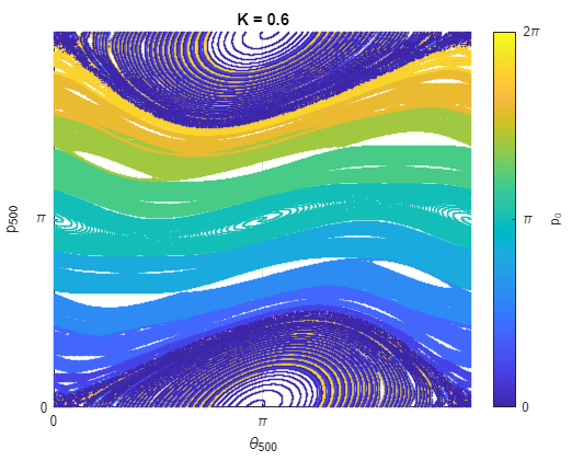
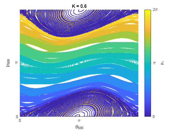
Run the simulations on your local machine for K=0.6 and plot the results.

K = 0.6;
if canUseGPU
    K = gpuArray(K);
end
[pN,thetaN] = simulateRotator(numKicks,numThetaValues,numPValues,K);
figure
plotMap(numKicks,pN,thetaN,K)

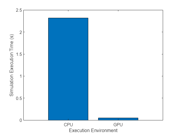
If you have a GPU on your local machine, check whether the simulations run faster on the GPU by timing the execution on the GPU and the CPU using the gputimeit and timeit functions respectively.

if canUseGPU
    gpu = gpuDevice;
    disp(gpu.Name + " GPU selected.")

    tGPU = gputimeit(@() simulateRotator(numKicks,numThetaValues,numPValues,K))
    K = gather(K);
    tCPU = timeit(@() simulateRotator(numKicks,numThetaValues,numPValues,K))
    
    disp("Speedup when running the simulations on a GPU compared to CPU: " + round(tCPU/tGPU) + "x")

    figure
    executionEnvironment = ["CPU" "GPU"];
    bar(executionEnvironment,[tCPU tGPU])
    xlabel("Execution Environment")
    ylabel("Simulation Execution Time (s)")
end

NVIDIA RTX A5000 GPU selected.

tGPU = 0.0517

tCPU = 2.3159

Speedup when running the simulations on a GPU compared to CPU: 45x

Setup Cluster

This example uses a MATLAB Parallel Server cluster created using Cloud Center. Cloud Center provides an easy way to create and manage cloud computing resources and access them through MATLAB. Once you have created a cluster, you can discover it by using the Discover Clusters button. For more information on creating MATLAB Parallel Server clusters using Cloud Center, see Create and Discover Clusters.

Create a cluster object. In this example, the Cloud Center cluster is named cloudCenterCluster and has four machines, each with a single GPU.

c = parcluster("cloudCenterCluster");

Create Pool and Check GPUs

Create a parallel pool a number of workers equal to the number of GPUs in the cluster. Alternatively, to use a batch workflow to offload work to the cluster, for example using batch, you do not need to create a parallel pool.

gpusInCluster = 4;
pool = parpool(c,gpusInCluster);

Starting parallel pool (parpool) using the 'cloudCenterCluster' profile ...
Connected to parallel pool with 4 workers.

You can use the gpuDevice and gpuDeviceTable functions to inspect GPUs on your local machine. If your local machine does not have a supported GPU, calls to gpuDevice error and calls to gpuDeviceTable return an empty table. To run these functions on the cluster machines, you can run them inside an spmd block (or another parallel language feature that runs code on multiple workers, such as parfor, or parfeval). You can distinguish GPUs with the same name by inspecting their universally unique identifier (UUID). Verify that the parallel pool has access to the GPUs.

spmd
    gpu = gpuDevice;

    disp("GPU: " + gpu.Name)
    disp("UUID: " + gpu.UUID)
end

Worker 1:
  GPU: A10G
  UUID: GPU-e7c907df-338a-f20c-5fd1-e79bdd519955
Worker 2:
  GPU: A10G
  UUID: GPU-400fdbba-fbff-7be8-9b7d-c61404c48227
Worker 3:
  GPU: A10G
  UUID: GPU-aafc0b00-89b6-702c-3d0e-6c3aacdfc9d2
Worker 4:
  GPU: A10G
  UUID: GPU-813c3257-e0dc-93a5-d949-4988fe7dcabf

Run Simulations on Remote GPUs

After you have created a parallel pool, you can use any of the interactive parallel language constructs provided by MATLAB, for example, parfor, parfeval, and spmd. As each simulation is independent of all of the others in this example, parfor is a good a choice. For more information on choosing between parallel computing language features, see Parallel Language Decision Tables.

Use a parfor-loop to offload the simulation calculation to the parallel workers and return the simulation results to the client session and time the parfor-loop.

K = 0:0.1:3;
KTrials = numel(K);

parfor idx = 1:KTrials
    gpuK = gpuArray(K(idx));
    [pN,thetaN] = simulateRotator(numKicks,numThetaValues,numPValues,gpuK);

    pOut(:,:,idx) = pN;
    thetaOut(:,:,idx) = thetaN;
end

Analyzing and transferring files to the workers ...done.

The output arrays pOut and thetaOut contain gpuArray data. If your local machine has a supported GPU, you can immediately access and use this data in the client MATLAB session. If your local machine does not have a supported GPU, call gather before using it in subsequent code.

pOut = gather(pOut);
thetaOut = gather(thetaOut);

Plot Results

Plot the results for each value of K and capture each plot in a frame.

F(KTrials) = struct("cdata",[],"colormap",[]);
fig = figure(Visible="off");

parfor idx=1:KTrials   
    plotMap(numKicks,pOut(:,:,idx),thetaOut(:,:,idx),K(idx))
    F(idx) = getframe(fig);
end

Play the sequence of frames.

fig = figure(Visible="on");
movie(fig,F)

Supporting Functions

simulateRotator

The simulateRotator function simulates a kicked rotator for numKicks kicks of intensity K, for a number of initial angular position and angular moment values numThetaValues and numPValues. If K is a gpuArray, then the function performs the simulations on the GPU. Otherwise, the function performs the simulations on the CPU.

function [pN,thetaN] = simulateRotator(numKicks,numThetaValues,numPValues,K)

% Create initial values of p and theta. If K is a gpuArray, create p and theta on the GPU.
zero = zeros(like=K);
p = linspace(zero,(numPValues-1)*2*pi/numPValues,numPValues);
theta = linspace(zero,2*pi,numThetaValues);

[p,theta] = ndgrid(p,theta);

for i=1:numKicks
    p = p + K*sin(theta);
    theta = theta + p;
end

% Modulo 2pi.
p = mod(p,2*pi);
theta = mod(theta,2*pi);

% Convert the final values p and theta to single.
pN = single(p);
thetaN = single(theta);

end

plotMap

The plotMap function plots $\theta {}_{\mathit{n}}$ and ${\mathit{p}}_{\mathit{n}}$, and colors each point according to its initial angular momentum ${\mathit{p}}_0$.

function plotMap(numKicks,p,theta,K)

% Color points by initial value of p.
[numPValues,numThetaValues] = size(p);
c = linspace(0,2*pi,numPValues+1);
c(end) = [];
c = repmat(c,1,numThetaValues);

% Plot final p and theta in a scatter plot.
scatter(theta(:),p(:),1,c(:),"filled")


% Add title and axes labels.
title("K = " + gather(K))
xlabel("\theta_{"+numKicks+"}")
ylabel("p_{"+numKicks+"}")
xticks([0 pi 2*pi])
yticks([0 pi 2*pi])
xticklabels(["0" "\pi" "2\pi"])
yticklabels(["0" "\pi" "2\pi"])
xlim([0 2*pi])
ylim([0 2*pi])
grid on

% Add color bar.
cBar = colorbar(Ticks=[0 pi 2*pi],TickLabels={"0" "\pi" "2\pi"});
cBar.Label.String = "p_0";
clim([0 2*pi])

end