2-D Slices Through 3-D Geometry with MATLAB Functions

R2026b

This example shows how to obtain plots from 2-D slices through a 3-D geometry. Here, you find and plot the temperature distribution on a square plate when a laser beam hits the middle of the plate and generates a heat flux.

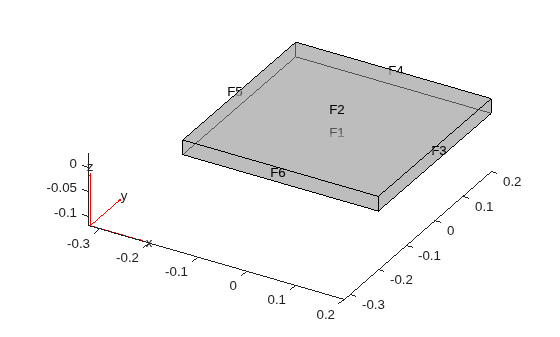
Create and plot a geometry representing a 40-by-40-by-3 cm plate.

L = 0.4; % m
W = 0.4; % m
H = 0.03; % m
g = multicuboid(L,W,H);
pdegplot(g,FaceLabels="on",FaceAlpha=0.5)

Create a finite element analysis model for transient thermal analysis and include the plate geometry.

model = femodel(AnalysisType="thermalTransient", ...
                Geometry=g);

Generate a mesh.

model = generateMesh(model,Hmax=H/4);

Specify the material properties and the initial temperature of the plate.

model.MaterialProperties = ...
    materialProperties(ThermalConductivity=50, ...
                       MassDensity=1960, ...
                       SpecificHeat=710);
model.CellIC = cellIC(Temperature=300);

Specify the heat flux boundary condition on top of the plate. First, specify a heat flux as a short pulse created by the laser beam by using the heatFluxSteady function.

function fluxValSteady = heatFluxSteady(location,state)
A = 350000000;
x0 = 0;
y0 = 0;
sx = 0.1; % standard deviation along x
sy = 0.05; % standard deviation along y

fluxValSteady = A*exp(-(((location.x-x0).^2/(2*sx^2))+ ...
                        ((location.y-y0).^2/(2*sy^2))));

% Beam switches off after 0.03 seconds
    if state.time > 0.03   
        fluxVal = 0*location.x;
    end
end

model.FaceLoad(2) = faceLoad(Heat = @heatFluxSteady);

Solve the thermal problem for the times between 0 and 2 seconds.

tlist = 0:0.5:2;
results = solve(model,tlist);

Plot the temperature distribution on the surface of the plate for the last time step by using the pdeplot3D function.

pdeplot3D(results.Mesh, ...
          ColorMapData=results.Temperature(:,end))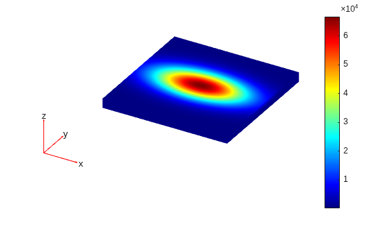

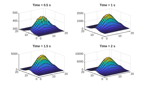
Now plot the slice through the solution showing the temperature distribution under the surface of the plate. Create a grid of (x,y,z) points, where x and y correspond to the length and width of the plate, and z is three quarters the thickness of the plate. Interpolate temperatures to these grid points and all times.

xx = -L/2:L/20:L/2;
yy = -W/2:W/20:W/2;
[XX,YY] = meshgrid(xx,yy);
ZZ = 3/4*H*ones(size(XX));
Tintrp = interpolateTemperature(results,XX,YY,ZZ,1:length(tlist));

The solution matrix Tintrp has five columns, one for each time in tlist.

size(Tintrp)

ans = 1×2

   441     5

Plot the temperature distribution for each time, excluding the initial time 0. Reshape the temperature vectors and make a surface plot of each temperature distribution by using the surf function.

figure
tiledlayout('flow');
for t = 2:length(tlist)
    nexttile
    Tsol = Tintrp(:,t);
    Tsol = reshape(Tsol,size(XX));
    surf(Tsol)
    title({['Time = ' num2str(tlist(t)) ' s']})
end

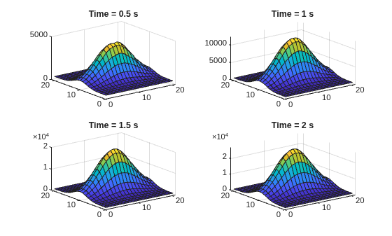
For comparison, interpolate and plot the temperature distribution halfway through the plate thickness.

ZZ = 0.5*H*ones(size(XX));
Tintrp = interpolateTemperature(results,XX,YY,ZZ,1:length(tlist));

figure
tiledlayout('flow');
for t = 2:length(tlist)
    nexttile
    Tsol = Tintrp(:,t);
    Tsol = reshape(Tsol,size(XX));
    surf(Tsol)
    title({['Time = ' num2str(tlist(t)) ' s']})
end