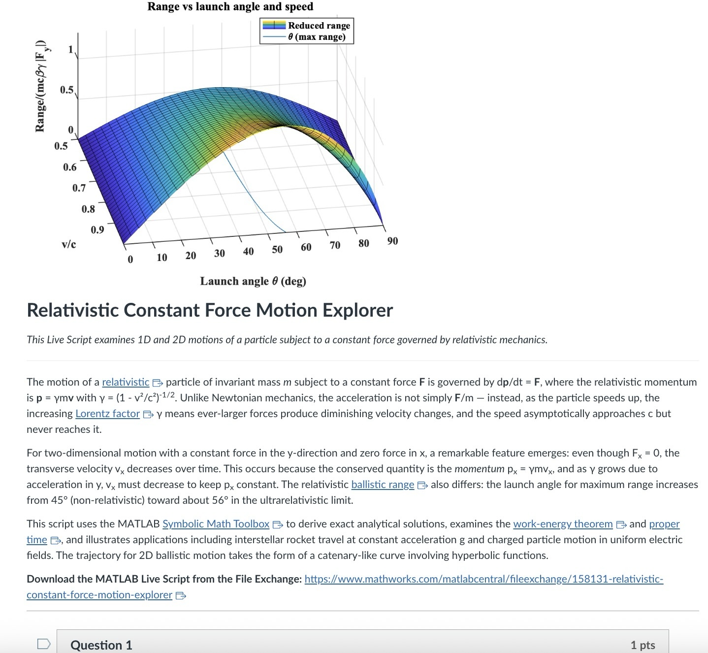
Results for
talks about how GeForce has become deprioritized by Nvidia, and
The chatter from the grapevine is that we won't see any new GPUs from Nvidia this
year at all — not one — and that's very rare (in fact it hasn't happened in three
decades). This is because Nvidia needs all the chips it can get — and perhaps more
to the point, all the video RAM — for AI graphics cards which are far more
profitable than consumer models.
Soon, Mathworks will be facing a choice: continue to support only expensive Nvidia AI offerings -- or diversify to support alternative GPUs as well.
By the way: Nvidia AI units cost $US7.8 million dollars. https://www.tomshardware.com/tech-industry/artificial-intelligence/nvidias-memory-costs-soar-485-percent-latest-ai-systems-now-cost-usd7-8-million-to-build-memory-now-comprises-25-percent-of-the-total-cost-rubin-gpus-a-mere-usd50-000-apiece
Which alternative GPUs would you most like to see supported?
- Unfortunately, I hear that Apple provides poor support for information on really using their "silicon" GPUs in any way other than Apple's pre-packaged computation libraries. The Apple attitude is apparently that anything that is not already nailed down by documentation is fair game for changing in the future, and that documenting how the GPUs really work would constitute nailing them down, supposedly "destroying" Apple's creativity. Exception: Apple is known to work with major gaming studios (but only the major ones.)
- The Apple silicon series of GPU does not provide any 64 bit operations, so 64 bit support would require emulating 64 bits in software. Nvidia is famous for internally implementing 64 bit support in terms of 32 bit operations, at 1:32 of the speed -- but on the other hand select Nvidia devices operate 64 bit operations at 1:24 or even 1:8 (a small number of devices) through hardware acceleration units. People who need 64 bit operations have the option of shopping very carefully in Nvidia's line to get faster 64 bit processing.
- OpenCL sounds cool and "open". Unfortunately it turns out that a lot of OpenCL operations are optional, so efficient OpenCL libraries would need to be tuned to the exact hardware series.
- OpenCL is not supported on semi-recent MacOS Intel or Apple Silicon series
- I seem to recall hearing that OpenCL is no longer supported by Nvidia either
Background: I've been using Claude Code with the MATLAB MCP Core Server and Simulink Agentic Toolkit for powertrain simulation work — building PMSM FOC controllers, Simscape thermal models, and suspension systems. After a few sessions I noticed a large fraction of my context window was being consumed by output that's useful to a human but not to an LLM: aligned whos tables, repeated solver warnings (one per timestep), deep call stacks with HTML hyperlinks, Simulink build logs, etc.
What I built: A transparent Python stdio proxy that sits between Claude Code and matlab-mcp-core-server. It intercepts tool responses and applies 14 MATLAB/Simulink/Simscape-specific compression rules before the output reaches Claude's context window. Requests are never touched — only responses.
Example reductions:
- whos variable table → 74% reduction (1,800 chars → 189 chars)
- Repeated solver warnings (×10 RCOND warnings) → 71% reduction
- Large array auto-display (1000-row vector) → 85% reduction
- Simulink build log → 56% reduction
- DOE progress loop (55 points) → 79% reduction
- Session average: 48–66% reduction
It also fixes the simulink session attach problem. Without --initialize-matlab-on-startup=true on the matlab server, the simulink server's 30-second discovery window expires before MATLAB is ready. The proxy config includes this flag and documents why it's necessary (root cause traced through server logs).
Validated on: A 2-DOF Simscape quarter-car active suspension model built entirely via model_edit from the SATK — active PD controller achieved 61.7% lower peak chassis velocity and settled 34% faster than passive.
Includes 37 unit tests, full HTML documentation, and the validated Simscape model. Would be interested to hear if others have run into the same output verbosity issues and what workarounds you've tried.
Prototyping MATLAB code in Claude's container with Octave
Duncan Carlsmith, Department of Physics, University of Wisconsin-Madison

Fig. 1: Simulated rigid molecules trajectories
When working with AI to develop MATLAB code for a chaotic-dynamics simulator, I discovered a useful workflow trick: Claude's container ships with GNU Octave. Claude can write .m files and execute them directly, as it can Python, getting fast feedback before you ever push to your local system. The related workflow described here may be possible using any agentic AI offering access to Octave.
The code simulates a classical 2D monatomic or diatomic (rigid or flexible) molecule undergoing a volume compression and compares the adiabatic coefficient in the simulation to the predictions of the ideal gas model and classical thermodynamics, assuming equipartition of energy between the translational, rotational, and vibrational degrees of freedom. Energy is injected by the moving container wall to various degrees of freedom during collisions, and the goal is to see how well the degrees of freedom thermalize through wall collisions alone without intermolecular collisions, and to study wall shape effects. The simulation uses an impact dynamics model for the collisions and tightly controlled state propagation.
My setup includes Claude, an ngrok link to speed up file transfer between a chat container and my local file system, and MATLAB MCP, enabling Claude to push and run MATLAB R2025b and collect output. I decided to first develop in Python entirely in the container, telling Claude to think in advance about porting to MATLAB. This approach allowed Claude to debug quite a package of Python code without the overhead of transferring code and results to and from my system. At various stages, we backed up the Python along with status reports to my filesystem in case the chat failed.
The next stage was to port to MATLAB. When Claude just launched into testing the MATLAB code with Octave in its container, I was taken aback - I hadn’t ever thought of that or known it was a built-in option. We proceeded to make floating-point comparisons of the Python and Octave simulation outputs (which agreed to ~1e-13) to debug the Octave. Finally, we simply transferred about 30 files of Octave/MATLAB code to my filesystem and verified it worked.
The version problem
Claude's container runs Octave 8.4.0, released in late 2023. The current Octave is 11.1.0, released February 2026. Octave is actively maintained, with three or four releases per year. Newer classdef improvements, advances with sparse/diagonal matrices, and various function flags available in 11.1 are lacking in 8.4. For my simulation code, none of this turned out to matter.
Why not just upgrade?
According to Claude, “the container is Ubuntu 24.04 LTS, and its repositories only offer 8.4.0. A standard apt-get install chain failed in interesting ways — Ubuntu's security archive sometimes drops point-version .deb files that the local package index still references, breaking unrelated dependency chains. The openssh-client package got 404'd, which cascaded through openmpi-bin, stopping the install.” Claude suggested “building from source (45+ minutes of compile, plus C++20 and Fortran toolchains), a third-party PPA, or Flatpak (which isn't installed).” My answer was: “I don’t understand all that gobbledygook. Live with 8.4, but write code that will also work in modern MATLAB.”
Octave 8.4 handles array operations, slicing, broadcasting, structs, .mat file I/O via load/save, anonymous functions, fzero and other root-finders, ODE solvers, +package/ namespace folders, sparse matrices, and basic plotting. For our project — a wall-collision simulator with a Forest-Ruth symplectic integrator and Brent's method root-finding — every line of Python code ran identically in MATLAB. The numerical answers differed at the floating-point-precision level (Octave's fzero and MATLAB's fzero round slightly differently, apparently).
Gotchas
A few pitfalls were encountered that you might note if you try this workflow.
1. Nested function definitions inside loops or after executable code
Octave is relaxed about where you put helper function blocks. MATLAB R2025b is strict: local functions go at the end of a file, not inside another function body or — fatally — inside a for loop. I had written:
for i = 1:n
if condition
function f = f_trial(t) % LEGAL in Octave, ERROR in MATLAB
...
end
root = fzero(@f_trial, ...);
end
end
MATLAB rejected this with "Function definition is misplaced or improperly nested." The fix is to move helpers to the end of the file as proper local functions, and use anonymous functions for closures over loop-local variables:
for i = 1:n
if condition
r0 = snapshot_r; % capture in loop scope
f_trial = @(t) helper(t, r0, ...); % captures at creation
root = fzero(f_trial, ...);
end
end
function f = helper(t, r0, ...) % at file end
...
end
2. MATLAB's arguments...end validation block
A MATLAB feature for argument typing and defaults is unsupported in Octave. The modern MATLAB style:
function log = simulate(state, schedule, opts)
arguments
state struct
schedule struct
opts.N_max (1,1) double = 200000
opts.verbose (1,1) logical = false
end
% opts.N_max and opts.verbose available, types and sizes validated
...
end
Octave's parser doesn't recognize the arguments keyword. The fallback is old-style manual parsing:
function log = simulate(state, schedule, varargin)
N_max = 200000;
verbose = false;
for k = 1:2:numel(varargin)
switch varargin{k}
case 'N_max', N_max = varargin{k+1};
case 'verbose', verbose = varargin{k+1};
end
end
...
end
3. Hardcoded paths
Not an Octave-specific problem, but Claude's container has different paths than your local filesystem. Resolve data files relative to the script:
this_dir = fileparts(mfilename('fullpath'));
data = load(fullfile(this_dir, 'comparison', 'data.mat'));
4. Variable name collision
Again, not an Octave-specific problem, but variable name collisions (with Python objects in your workspace, or stale function caches after Claude pushes a new file) can cause confusing errors. clear all resets both.
5. Floating-point differences that get amplified
Octave's fzero and MATLAB's fzero round differently. In chaotic dynamics, such differences can be amplified. For the simulator we built, the same flexible molecule initial condition ran to 215 collisions in Octave and 226 in MATLAB R2025b — identical physics, different trajectories. That such tiny differences could be amplified in this simulation was verified with tests in the three languages - Python, Octave, and MATLAB.
Speed
Claude pointed out that performance varies with language and offered a comparison for a flexible molecule example with ~215-230 wall collisions): Python (CPython 3 + NumPy + scipy.brentq), ~3.3 s, 1×;MATLAB R2025b, 0.5 s, 0.15× (6.6x faster than Python); Octave 8.4 in Claude's container, ~10 s, 3× (3x slower than Python).
In this most challenging case, the integrator has to step between collisions to properly simulate the coupled rotations and vibrations. The 20x speed improvement of MATLAB over Octave might be due to the MATLAB JIT.
Conclusion
When I first started developing MATLAB Live Scripts for physics education, I suggested Octave as an open-source alternative for those educators who had no MATLAB site license. Knowing the limitations of Octave and not knowing if its development would continue, I have not limited myself to Octave-compatible code. I am nonetheless tickled that this workflow succeeded. I might have skipped the Python prototype for this project. Of course, for those projects featuring MATLAB toolboxes not supported by Octave or Python, prototyping MATLAB code in these languages is more complicated.
Conflict of interest
The author declares he has no financial interest in Mathworks or Anthropic. This article is informational and does not constitute an endorsement by the University of Wisconsin-Madison of any vendor or product. Claude is a trademark of Anthropic. MATLAB is a trademark of Mathworks.
I am a bit neurotic about getting things "just right" and I would really like the ability to resize panels on the desktop to predefined default configurations. I know that I can set up the panels by hand and save them, but I'd like to be able to automatically set a 3 column layout to 25%-50%-25% or perhaps 33%-34%-33% This would be somewhat like the snap feature in windows shown here: https://support.microsoft.com/en-us/windows/snap-your-windows-885a9b1e-a983-a3b1-16cd-c531795e6241. This wouldn't have to preclude setting them by hand but it would offer an automated alternative.
If this feature already exists, perhaps someone can point me to it.
Have been using Thingspeak for a few years, suddenly I get this message relating to one of my Matlab analysis scripts, which has run for years:
Error Message:
Unrecognized function or variable 'cusum'. cusum requires Signal Processing Toolbox.
What has changed to cause this error - I've done nothing!

Generate a 3D visualization of carnation flowers
with sepals and stems for celebrating Mother's Day 2026.

function carnation
% CARNATION Generate a 3D visualization of carnation flowers with sepals and stems.
% This code is authored by Zhaoxu Liu / slandarer
% for the purpose of celebrating Mother's Day 2026.
% =========================================================================
% Zhaoxu Liu / slandarer (2026). carnation for Mother's Day
% (https://www.mathworks.com/matlabcentral/fileexchange/183838-carnation-for-mother-s-day),
% MATLAB Central File Exchange. Retrieved May 9, 2026.
% Create figure and axes / 创建图窗及坐标区域
fig = figure('Units','normalized', 'Position',[.3,.1,.4,.8],'Color',[244,234,225]./255);
axes('Parent',fig, 'NextPlot','add', 'DataAspectRatio',[1,1,1],...
'View',[-64, 5.5], 'Position',[0,-.15,1,1], 'Color',[244,234,225]./255, ...
'XColor','none', 'YColor','none', 'ZColor','none');
annotation("textbox", [.05, .8, .9, .2], "String", {"Happy"; "Mother's Day"}, ...
'FontName','Segoe Script', 'FontSize',52, 'FontWeight','bold', 'EdgeColor','none', ...
'HorizontalAlignment','center', 'VerticalAlignment','middle', 'Color',[97,40,20]./255);
xx = linspace(0, 1, 100);
tt = linspace(0, 1, 1e4);
[X, P] = meshgrid(xx, tt);
T1 = P*20*pi;
C1 = 1 - (1 - mod(3.6*T1/pi, 2)).^4./2; % Petal profile / 花瓣形状
S1 = (sin(50*T1)/150 + sin(10*T1)/30).*min(1, max(0, (X - .85)/.1)); % Edge serration / 边缘褶皱和锯齿
Y1 = (- (X.*1.2 - .5).^5.*32 - 1)./15.*P; % Petal curvature / 花瓣弧度
% Petal shape and serration modeling + rotating the planar petal to tilt it
% 花瓣形状和锯齿塑造 + 转动平躺的花瓣令其倾斜
R1 = (C1 + S1).*(X.*sin(P) - Y1.*cos(P))./(P + .5);
H1 = (C1 + S1).*(X.*cos(P) + Y1.*sin(P));
% Convert radius to Cartesian coordinates / 将半径映射为X,Y坐标
X1 = R1.*cos(T1);
Y1 = R1.*sin(T1);
% Colormap for carnation petals / 康乃馨配色
CList1 = [208, 62, 23; 221,146,121; 229,201,202; 233,219,222; 237,223,225]./255;
CMat1 = zeros(1e4, 100, 3);
CMat1(:, :, 1) = repmat(interp1(linspace(0, 1, size(CList1, 1)), CList1(:, 1), linspace(0, 1, 100)), [1e4, 1]);
CMat1(:, :, 2) = repmat(interp1(linspace(0, 1, size(CList1, 1)), CList1(:, 2), linspace(0, 1, 100)), [1e4, 1]);
CMat1(:, :, 3) = repmat(interp1(linspace(0, 1, size(CList1, 1)), CList1(:, 3), linspace(0, 1, 100)), [1e4, 1]);
% Darken edges / 边缘的深色
for i = 1:1e4
tNum = randi([98, 100]);
CMat1(i, tNum:end, 1) = 212./255;
CMat1(i, tNum:end, 2) = 87./255;
CMat1(i, tNum:end, 3) = 113./255;
end
% Rotation matrices / 旋转矩阵
Rx = @(rx) [1, 0, 0; 0, cos(rx), -sin(rx); 0, sin(rx), cos(rx)];
Rz = @(yz) [cos(yz), - sin(yz), 0; sin(yz), cos(yz), 0; 0, 0, 1];
Rx1 = Rx(pi/6); Rz1 = Rz(0);
% Render flower / 绘制康乃馨
surface(X1, Y1, H1 + .3, 'CData',CMat1, 'EdgeAlpha',0.1, 'EdgeColor',[224,39,39]./255, 'FaceColor','interp')
[U1, V1, W1] = matRotate(X1, Y1, H1 + .3, Rx1);
surface(U1 + .7, V1 - .7, W1 - .6, 'CData',CMat1, 'EdgeAlpha',0.1, 'EdgeColor',[224,39,39]./255, 'FaceColor','interp')
% Following the same method as before,
% the profile is designed with four serrated cycles to simulate the four sepals.
% 还是之前的方法,不过让轮廓有4个锯齿状周期来模拟四片花萼
% Sepals generation with 4-lobed pattern / 生成四片花萼(带4个锯齿状周期)
[X, T] = meshgrid(linspace(0, 1, 100), linspace(0, 1, 100).*2*pi);
P2 = T.*0 + pi/8;
C2 = .5 + (.5 - abs(mod(T, pi/2)/pi*2 - .5))*.4;
Y2 = (- (X.*1 - .5).^7.*128 - 1)./15 - .1;
R2 = C2.*(X.*sin(P2) - Y2.*cos(P2));
H2 = C2.*(X.*cos(P2) + Y2.*sin(P2));
X2 = R2.*cos(T);
Y2 = R2.*sin(T);
% Rotate by 90 degrees around the z-axis
% and reduce the size to render the four smaller sepals.
% 绕z轴旋转90度且减小其大小,绘制四片小花萼
% Smaller sepal layer / 绘制四片小花萼(第二层)
P3 = T.*0 + pi/10;
C3 = .3 + (.5 - abs(mod(T + pi/4, pi/2)/pi*2 - .5))*.7;
Y3 = (- (X.*.7 - .5).^7.*128 - 1)./15 - .1;
R3 = C3.*(X.*sin(P3) - Y3.*cos(P3));
H3 = C3.*(X.*cos(P3) + Y3.*sin(P3));
X3 = R3.*cos(T);
Y3 = R3.*sin(T);
% Colormap for sepals / 花托配色
CList2 = [178,173,113; 151,135, 73; 117,123, 50; 86, 89, 29; 75, 65, 17]./255;
CMat2 = zeros(100, 100, 3);
CMat2(:, :, 1) = repmat(interp1(linspace(0, 1, size(CList2, 1)), CList2(:, 1), linspace(0, 1, 100)), [100, 1]);
CMat2(:, :, 2) = repmat(interp1(linspace(0, 1, size(CList2, 1)), CList2(:, 2), linspace(0, 1, 100)), [100, 1]);
CMat2(:, :, 3) = repmat(interp1(linspace(0, 1, size(CList2, 1)), CList2(:, 3), linspace(0, 1, 100)), [100, 1]);
% Render sepals / 绘制花托
surf(X2, Y2, H2.*.8 + .12, 'CData',CMat2, 'EdgeAlpha',0.1, 'EdgeColor',CList2(end,:), 'FaceColor','interp')
surf(X3.*.93, Y3.*.92, H3.*.5 + .02, 'FaceColor',[ 84, 85, 54]./255, 'EdgeAlpha',0.1, 'EdgeColor','k')
[U2, V2, W2] = matRotate(X2, Y2, H2.*.8 + .12, Rx1);
[U3, V3, W3] = matRotate(X3.*.93, Y3.*.92, H3.*.5 + .02, Rx1);
surf(U2 + .7, V2 - .7, W2 - .6, 'CData',CMat2, 'EdgeAlpha',0.1, 'EdgeColor',CList2(end,:), 'FaceColor','interp')
surf(U3 + .7, V3 - .7, W3 - .6, 'FaceColor',[ 84, 85, 54]./255, 'EdgeAlpha',0.1, 'EdgeColor','k')
% A pulse function with two periods is applied
% to the contour to simulate the leaves.
% 让轮廓有2个周期且是脉冲函数,来模拟叶片
P4 = T.*0 + pi/16;
C4 = - abs(mod(T, pi)/pi - .5) + .11;
C4(C4 < 0) = 0; C4 = C4.*10; C4(51:100, :) = C4(51:100, :).*.7;
Y4 = (- (X.*1.01 - .5).^7.*128 - 1)./15 - .03;
R4 = C4.*(X.*sin(P4) - Y4.*cos(P4));
H4 = C4.*(X.*cos(P4) + Y4.*sin(P4));
X4 = R4.*cos(T);
Y4 = R4.*sin(T);
surf(X4 - .1, Y4 + .05, H4 - 2.2, 'FaceColor',[ 84, 85, 54]./255, 'EdgeAlpha',0.1, 'EdgeColor','k')
[U4, V4, W4] = matRotate(X4 - .1, Y4 - .1, H4 + .1, Rz1);
[U4, V4, W4] = matRotate(U4, V4, W4, Rx1);
surf(U4 + .7, V4 - .7 + 1, W4 - .6 - 1.2, 'FaceColor',[ 84, 85, 54]./255, 'EdgeAlpha',0.1, 'EdgeColor','k')
P5 = T.*0 + pi/8;
C5 = - abs(mod(T + pi/6, pi)/pi - .5) + .11;
C5(C5 < 0) = 0; C5 = C5.*5;
Y5 = (- (X.*1.01 - .5).^7.*128 - 1)./15 - .1;
R5 = C5.*(X.*sin(P5) - Y5.*cos(P5));
H5 = C5.*(X.*cos(P5) + Y5.*sin(P5));
X5 = R5.*cos(T);
Y5 = R5.*sin(T);
surf(X5, Y5, H5 - .3, 'FaceColor',[ 84, 85, 54]./255, 'EdgeAlpha',0.1, 'EdgeColor','k')
[U5, V5, W5] = matRotate(X5, Y5, H5+.1, Rx1);
surf(U5 + .7, V5 - .7 + 1/4, W5 - .6 - 1.7/4, 'FaceColor',[ 84, 85, 54]./255, 'EdgeAlpha',0.1, 'EdgeColor','k')
% Render stems / 绘制花杆
P1_1 = [mean(X3(:).*.93), mean(Y3(:).*.92), mean(H3(:).*.5 + .02)];
P1_2 = [mean(X5(:)), mean(Y5(:)), mean(H5(:) - .3)];
P1_3 = [mean(X4(:) - .1), mean(Y4(:) + .05), mean(H4(:) - 2.2)];
P1_3 = (P1_3 - P1_2).*1.4 + P1_2;
[XX1, YY1, ZZ1] = cylinderXYZ(P1_1, P1_2, .05);
[XX2, YY2, ZZ2] = cylinderXYZ(P1_2, P1_3, .04);
surf(XX1, YY1, ZZ1, 'FaceColor',[ 84, 85, 54]./255, 'EdgeAlpha',0.1, 'EdgeColor','k')
surf(XX2, YY2, ZZ2, 'FaceColor',[ 84, 85, 54]./255, 'EdgeAlpha',0.1, 'EdgeColor','k')
P1_1 = [mean(U3(:) + .7), mean(V3(:) - .7), mean(W3(:) - .6)];
P1_2 = [mean(U5(:) + .7), mean(V5(:) - .7 + 1/4), mean(W5(:) - .6 - 1.7/4)];
P1_3 = [mean(U4(:) + .7), mean(V4(:) - .7 + 1), mean(W4(:) - .6 - 1.2)];
P1_3 = (P1_3 - P1_2).*2.4 + P1_2;
[XX1, YY1, ZZ1] = cylinderXYZ(P1_1, P1_2, .05);
[XX2, YY2, ZZ2] = cylinderXYZ(P1_2, P1_3, .04);
surf(XX1, YY1, ZZ1, 'FaceColor',[ 84, 85, 54]./255, 'EdgeAlpha',0.1, 'EdgeColor','k')
surf(XX2, YY2, ZZ2, 'FaceColor',[ 84, 85, 54]./255, 'EdgeAlpha',0.1, 'EdgeColor','k')
% 在任意两点间构建圆柱
function [XX, YY, ZZ] = cylinderXYZ(P1, P2, r)
% CYLINDERXYZ Create a cylinder connecting two 3D points
% [XX, YY, ZZ] = cylinderXYZ(P1, P2, r) generates a cylinder
% of radius r between points P1 and P2.
v = P2 - P1; l = norm(v);
if l < eps, return; end
[XX, YY, ZZ] = cylinder(r, 30); ZZ = ZZ * l;
ddir = [0, 0, 1]; tdir = v / l;
if dot(ddir, tdir) > 0.9999
R = eye(3);
elseif dot(ddir, tdir) < -0.9999
R = [1, 0, 0; 0, -1, 0; 0, 0, -1];
else
av = cross(ddir, tdir); av = av / norm(av);
R = axisRotate(av, acos(dot(ddir, tdir)));
end
for ii = 1:size(XX, 1)
for jj = 1:size(XX, 2)
p = R * [XX(ii, jj); YY(ii, jj); ZZ(ii, jj)];
XX(ii, jj) = p(1) + P1(1);
YY(ii, jj) = p(2) + P1(2);
ZZ(ii, jj) = p(3) + P1(3);
end
end
end
% 通过矩阵旋转数据
function [U, V, W] = matRotate(X, Y, Z, R)
% MATROTATE Apply 3x3 rotation matrix to a set of 3D points
% [U,V,W] = matRotate(X,Y,Z,R) rotates points (X,Y,Z)
% using rotation matrix R.
U = X; V = Y; W = Z;
for ii = 1:numel(X)
v = [X(ii); Y(ii); Z(ii)];
n = R*v; U(ii) = n(1); V(ii) = n(2); W(ii) = n(3);
end
end
% 根据轴-角参数生成旋转矩阵
function R = axisRotate(axis, angle)
% AXISROTATE Compute rotation matrix from axis-angle representation
% R = axisRotate(axis, angle) returns a 3x3 rotation matrix
% for rotating by angle (radians) around the given axis vector.
% Implementation based on Rodrigues' rotation formula.
u = axis(1); v = axis(2); w = axis(3);
c = cos(angle); s = sin(angle);
R = [u^2 + (1-u^2)*c, u*v*(1-c) - w*s, u*w*(1-c) + v*s;
u*v*(1-c) + w*s, v^2 + (1-v^2)*c, v*w*(1-c) - u*s;
u*w*(1-c) - v*s, v*w*(1-c) + u*s, w^2 + (1-w^2)*c];
end
end
It turns out you can very easily change the list of verbs Claude Code uses to display when it's thinking. I've had fun replacing them with some MathWorks-specific verbiage. Comment below if you have any ideas to add to the list!
You just add the following to your settings.json file:
"spinnerVerbs": {
"mode": "replace",
"verbs": [
"MATLABing",
"Simulinking",
"MathWorking",
"MathWorkin' on it",
"Pre-allocating arrays",
"Checking 1-based indexing",
"Vectorizing",
"Eigenvaluing",
"FFT-ing",
"Transposing",
]
}
Hey AI, add computation to my modern physics course. Thanks.
Duncan Carlsmith
Department of Physics, University of Wisconsin-Madison
An AI-generated CANVAS quiz header based on a Live Script on relativistic motion.
Introduction
Agentic AI is disrupting higher education. An agentic AI can act on the web rather than relying solely on its training. It can research a topic and produce a credible research paper to specification with validated references. It can create, answer, or assess student work on physics questions from elementary mechanics to graduate-level quantum field theory or quantum computing. It can comprehend, generate, run, and debug a MATLAB Live Script zip package, an HTML5 interactive web application, a JavaScript-enabled website, an ADA-compliant CANVAS site with math and images, or a mobile phone app. A student can authenticate in a learning management system like CANVAS and issue a simple prompt to an agentic AI — “Complete all of my assignments in all of my courses. Thanks.” — and an instructor can, on the other side, with AI assistance and a simple prompt, assess all such submissions, even messy hand-written work. I have demonstrated these capabilities and others.
Here, I’d like to share an experiment leveraging AI to inject computation with MATLAB into a course in modern physics. This may interest the academic readers of this blog and the curious. My prior post Giving All Your Claudes the Keys to Everything introduced my personal agentic AI context.
Live Script goals
Some years back now, I started developing and introducing Live Scripts in a two-semester introductory physics course to immerse students in computation and science without sacrificing the rigor and breadth of the class. These students have essentially no background in computing and are exploring STEM majors — physics, astronomy, and engineering principally. A self-documenting Live Script allows a student to explore even a relatively advanced physics topic and data analysis trick like Fourier analysis or autocorrelation, using data like a mobile phone voice memo or a digital oscilloscope output race that they collect themselves, and then apply the same techniques to analyze big science open data from for example as gravitational wave observatory, both without being mired down in mathematics or code writing. As the course evolves, computational challenges connected to the laboratory component introduce much of the gamut of MATLAB functionality. The goal is to show why and how modeling and assessment using computation are essential in science, and to empower students with practical skills and a sense of what is possible. The traditional lecture/demonstration/homework/discussion format was largely untouched. This course sequence was a five-credit automatic honors course, so extra work was expected. Coding as a tool rather than a chore or vocation is all the more relevant in the AI age.
Assessment strategy
To flexibly direct and assess student work, each Live Script contains a variety of ‘Try this’ suggestions which require the user to adjust a parameter or two and observe the consequences. The student must study the physics described in the background information section, and the code enough to understand how the code logic works, using the supplied comments and URLs to documentation. Tackling a ‘Try this ‘ suggestion does not require any coding, just changing a parameter value, perhaps with a slider. Additionally, the Live Script contains ‘Challenges’ to extend the code in some simple or possibly advanced way. The Live Script can thus serve different customers, and an instructor can further tailor the script and embedded suggestions and challenges as they choose. The possibilities offered are only exemplary.
An associated CANVAS quiz contains a few multiple-choice questions related to the ‘Try this’ suggestions, which are auto-graded. Additional questions require the student to upload a product, like an appropriately labeled plot comparing data to a model fit, together with a written explanation. These are readily graded electronically using CANVAS SpeedGrader, with or without an e-rubric. The emphasis is on results and analysis, not on coding facility or style. By design, the burden on the instructor is minimal.
AI-generated computational thread
In teaching a 3-credit third-semester survey of modern physics (relativity, quantum mechanics, atomic, molecular, solid state, nuclear, particle, and astro physics) without a lab and again for students with little or no prior exposure to computation, I needed first to develop more advanced, relevant Live Scripts. This course offers three lecture hours per week, rife with live demonstrations of cathode ray tubes, electron diffraction, Geiger counters and sources, thermal radiation, the photoelectric effect, gas discharge tubes observed with diffraction glasses, lasers, and magnetic levitation with diamagnetic and high temperature superconductors, and so on. An additional mandatory hour per week is dedicated to small group active learning in sectional meetings. A contemporary e-text and integrated WebAssign homework system are linked via LTI to CANVAS. These components address learning goals I am loath to sacrifice. I ultimately decided to make the new computational thread an attractive extra-credit option (in parallel with a research paper option) and implemented it with AI assistance mid-stream this semester in a way that could be emulated.
The agent was Claude Desktop running with MCP servers: the Playwright browser-automation server (for CANVAS interaction via authenticated browser session), MATLAB MCP server to run MATLAB, and a filesystem server (for reading local Live Script packages and writing artifacts back to disk). I asked Claude to survey my modern physics syllabus on CANVAS and my 150+ Live Scripts on the MATLAB File Exchange (FEX), and to identify those relevant to a 3rd-semester course in relativity, quantum mechanics, atomic, molecular, solid state, nuclear, particle, and astro physics, with my Introduction to MATLAB script included as a foundations option. Claude returned an initial list of 38 candidate scripts. I removed two that were not a good fit and approved 14, including chaos in relativistic mechanics, relativistic motion in a Coulomb field, numerical solutions to the Schrödinger equation in 1D/2D/3D via the PDE Toolbox, gravitational-wave data analysis, exoplanet transit detection, and clustering in Gaia mission stellar data, among others.
For each approved script, Claude downloaded the FEX zip via MATLAB websave and unzip, converted the .mlx to readable .m text via matlab.internal.liveeditor.openAndConvert, ran the key numerical sections in MATLAB to obtain concrete answer values, and then used a single Playwright browser_evaluate call — authenticated by the CSRF token from the active CANVAS browser cookie — to POST a new quiz plus all of its questions to the CANVAS REST API in one round trip. (The MATLAB webwrite path with a CANVAS_API_TOKEN environment variable consistently returned 401 in our testing; the browser-session approach worked reliably for all 14 quizzes.)
Each quiz is structured identically: a description block with the FEX thumbnail image, a two- to three-paragraph physics introduction essentially copied from the FEX page or script itself with Wikipedia links to technical terms, a download link, and an “Open in MATLAB Online” link; followed by 4 multiple-choice questions worth 1 pt each (covering a fundamental physics fact, a physical mechanism, an experimental or computational technique, and a data-analysis concept), and 3 essay questions worth 3 pts each (a basic execution + screenshot, a quantitative comparison, and a bonus “Try this” modification). The essay type was deliberate: a CANVAS file_upload question accepts only a file, while an essay question gives the student a Rich Content Editor in which they can paste a screenshot directly from the clipboard and type their analysis in the same field. SpeedGrader then shows everything together. We also added an optional 0-credit student feedback question that we crafted jointly. Total: 13 points per quiz.
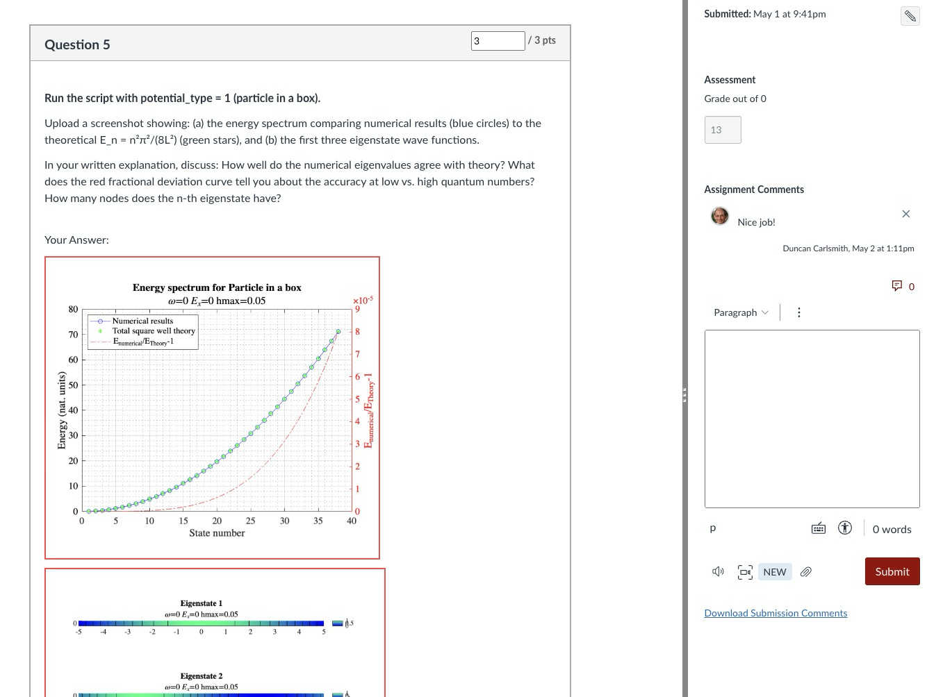
Speed Grader view of a Rich Content Editor question with uploaded results
The full set of 14 quizzes was created in a single working session. I reviewed and accepted the results essentially without revision — a few quiz descriptions needed a follow-up PUT to fix image sizing or to add the MATLAB Online link, but no question content required rewriting. Across the session, the procedure crystallized into a reusable SKILL.md that documents the FEX-to-CANVAS recipe end to end (download with MATLAB, design questions in the four-category MC pattern, batch quiz + question creation, verification checklist).
An AI touch on grading made the assignment fit the course without inflating its weight: a 5% group weight on the Computation category, with a drop-lowest-eleven-of-fourteen rule that keeps each student’s top three quizzes. Each quiz is 13 points, so the maximum contribution is (39/39) × 5% = 5.00% extra credit, and any student can attempt as few or as many as they wish without exceeding that cap. The CANVAS configuration is non-trivial in a few ways and includes one gotcha worth knowing about; details are in Appendix A.
Outcomes
I received about 75 submissions, with 30 of the 75 students participating, and many others opting for the research paper. Feedback was generally positive. Only a few students ran into difficulty: one suffered a European Space Agency network outage while accessing Gaia data, and another had trouble with a screen-capture process unrelated to MATLAB. Students reported workloads in an appropriate 1–3 hour range per assignment. Only about 20% of submitters elected to submit the (quite lengthy) Introduction to MATLAB assignment for credit; some likely encountered MATLAB already in the math department or engineering school, where it is used extensively, and others may have reviewed the assignment but elected not to submit because the upload questions concerned image processing (compression and decompression, blurring and deblurring) rather than course-relevant topics. Several students volunteered that these exercises were more informative and fun than their canonical problem-solving exercises.
Lessons
A few patterns from this experiment seem worth carrying forward. First, the ‘Try this’ design pattern that I had already adopted turns out to be unusually well suited to AI-assisted assessment: each suggestion converts almost mechanically into a three-part question (run, capture, analyze) with a defensible rubric; Hence one working session yielded a full term’s worth of quizzes. Second, the agentic build is a short, explicit recipe — read the script, run the calculations, design the questions, post via the CANVAS API in one batched call — that other instructors can replicate and which is now captured for me in a SKILL.md. Third, the Canvas grading mechanics (drop-lowest, keep-best-three, group weight cap) let extra-credit work scale gracefully: students self-select breadth versus depth, and the instructor’s exposure to grading volume is bounded.
Conclusions
More broadly, I expect education to become more efficient and engaging in this AI age, with much of the routine instructional and learning burden relegated to AI. Frontier AIs can affordably tutor undergraduate students and even PhDs at their level and challenge them in new ways and at scale. Students and instructors both must develop and adjust to new learning strategies and expectations. Documented exploration enabled by interactive, code-aware artifacts like Live Scripts and Jupyter notebooks, created by a student or researcher collaboratively with AIs and other compatriots, may play an ever more important role in this environment.
My SKILL.md is 665 lines and specific to my setup, so not shared here. You might be asking an AI to install Chromium and Playwright or Puppeteer and do all the work in its container. You might be electing a different assignment structure, accessing your own Live Scripts or Python equivalent located at GitHub or someplace other than the MATLAB FEX. This article documents most of what is in my skill file and would be useful background information. You will want to develop and test your own process if emulating the idea here.
Acknowledgements and disclosure
The products described here and this essay were prepared with the assistance of Claude.ai. The author declares he has no financial interest in Anthropic or MathWorks.
Appendix A: CANVAS gradebook configuration
The intent was simple to state: a student who completes three or more MATLAB quizzes at full marks should receive the full 5% extra-credit boost on their course total; a student who completes one quiz at full marks should receive one-third of that boost; a student who attempts none should receive nothing. Implementing this in CANVAS took three coordinated pieces, each of which is straightforward in isolation but has at least one non-obvious failure mode.
A.1 Group structure and drop rule. The 14 quizzes live in a single assignment group named “Computation,” weighted at 5% of the course grade. The group has one rule: drop the lowest 11 scores. With 14 assignments and 11 dropped, CANVAS keeps each student’s top three. Each quiz is worth 13 points (4 multiple-choice at 1 pt + 2 essay at 3 pts + 1 bonus essay at 3 pts), so the maximum sum across the kept three is 39, and the maximum group percentage is 39/39 = 100%, contributing 0.05 × 100% = 5.00% to the course total. The group weight thus acts as a hard ceiling: no matter how many quizzes a student attempts, their boost cannot exceed 5%.
A.2 Treating ungraded as zero, selectively. Out of the box, CANVAS treats ungraded assignments as ignored rather than as zero. This is usually the right default — a student who has not yet attempted an assignment is not penalized for it — but it interacts badly with the design intent here. If a student attempted exactly one MATLAB quiz and scored 13/13, CANVAS would show their Computation group total as 13/13 = 100%, awarding the full 5% boost for a single quiz. To get the intended scaling (one quiz at 13/13 should yield 13/39 = 33.33%, contributing 1.67% rather than 5%), the unattempted quizzes must count as zero in the group calculation.
The simplest way to enforce that globally is the gradebook setting Treat Ungraded as 0, but this applies course-wide and was undesirable in my case because of an exam-administration mixup in which different students had taken different versions of Exam 1; only the version each student took should count toward their exam grade, and a global “treat ungraded as 0” would have penalized students for the version they had not been assigned. The per-assignment alternative is to use the gradebook column menu (the three-dot menu on each assignment column) and choose Set Default Grade, entering 0 with the “Overwrite already-entered grades” box left unchecked. This converts every dash in that column to a 0 while leaving real scores untouched, and only affects the assignment whose menu was used. Applied to each of the 14 MATLAB quizzes, this gives the desired “ungraded as zero” behavior in the Computation group without affecting Exam 1 or any other category. After the fix, the worked examples behave as expected..
A.3 The points_possible gotcha. When a CANVAS Classic Quiz is created via the REST API and the quiz’s questions are POSTed in subsequent calls (or even, as in our case, in the same browser_evaluate call but as separate POST requests), the assignment row that mirrors the quiz in the gradebook can retain points_possible = 0 even though the questions internally sum to 13. The quiz preview displays the question points correctly, the quiz statistics show the correct totals, but the gradebook column header reads “Out of 0” and the group percentage calculation collapses to nonsense. Symptomatically, a student with one real score appeared at 30.77% in the Computation column when they should have been at 33.33% — the column was contributing 4/13 instead of 4/39 because 13 of the 14 columns were silently weightless.
The cure is to force CANVAS to recompute the assignment row’s points_possible from the question sum. The simplest way is per-quiz from the UI: open the quiz, click Edit, scroll to the bottom of the editor without changing anything, and click Save (not “Save & Publish” if the quiz is already published). The act of saving the quiz triggers the recompute. The same effect is available via the API by issuing PUT /api/v1/courses/{course_id}/assignments/{assignment_id} with body {"assignment": {"points_possible": 13}} on each affected assignment, which is faster for batch use.
The lesson for anyone scripting CANVAS quiz creation: after batch-creating quizzes and questions via the API, always verify the gradebook column header reads “Out of N” with N matching the question sum, and apply one of the two cures above before students start submitting. The skill file used in this project now flags this check explicitly.
Mitigating chat failures in AI code development
Duncan Carlsmith
Department of Physics, University of Wisconsin-Madison
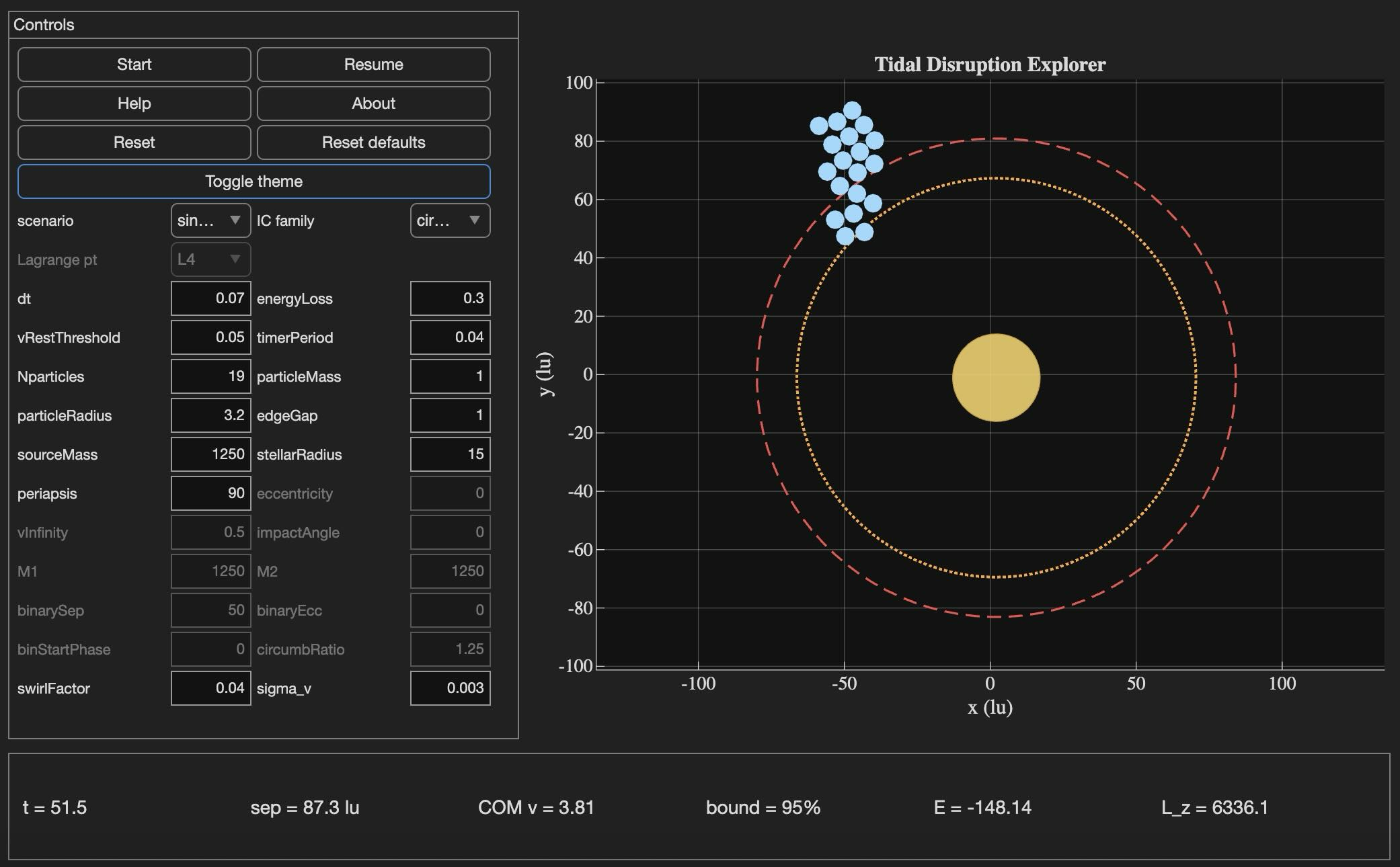
Tidal Disruption Explorer (MATLAB File Exchange 183760). The process of porting this Live Script ito HTML is described in this post.
Introduction
An agentic AI session ended for me this week with the message: "Claude is unable to respond to this request, which appears to violate our Usage Policy. Please start a new chat." Gulp. The substance of the conversation was completely benign — porting my MATLAB Live Script Tidal Disruption Explorer that simulates a self-gravitating cluster of particles being shredded by tidal forces near a massive object, like Comet Shoemaker-Levy 9 was shredded by Jupiter in 1992. The next chat picked up the work and finished it in seven turns.
Why nothing was lost is the subject of this post. The new product is the HTML5 port of Tidal Disruption Explorer and deployed at duncancarlsmith.github.io/TidalDisruptionExplorer-HTML5. But the more transferable product may be practices that can help make AI-assisted code development resilient to chat failures, connection drops, sandbox losses, and content-policy false positives. Two prior posts set my context: Live Script deployed as a 3D web application with AI introduced the workflow, and Giving All Your Claudes the Keys to Everything introduced the ngrok command server that makes the Mac controllable from any AI client. This post is about how to use such tools without losing your work when the chat dies.
Failure modes worth designing for
Long agentic sessions can fail in many ways, and most are out of the user's control. The bash_tool connection in the cloud container can go unresponsive mid-task. A stray Python process can mask a real command server on the same port. A lost development sandbox can vaporize generated artifacts — in an earlier turn of this same project, an entire test-harness directory disappeared with the sandbox and had to be reconstructed from the conversation log. Persistent context is not in fact persistent. Skills are forgotten. The user closes the laptop, the WiFi blinks off, or the chat hits a length limit. This project used Claude, but the problems are not AI-specific in my experience with 5-6 leading vendors. Without preparation, each of these is a real setback.
Best practices to consider
1. Externalize project state in a committed PROGRESS journal
A single file, committed in a repo, names every milestone, the test-pass count for each, the current state in prose, and an explicit "Recovery instructions for a fresh session" section that lists the source files, the test harness names, and the toolchain assumptions. When the previous chat failed, the next one resumed from this file alone, without needing the failed conversation. When the dev sandbox loss took out 10 test harnesses, they were rebuilt from the conversation log because the journal had recorded exactly what each harness checked and the expected pass count for each. These harnesses are also stored locally when complete and successful.
2. Two external locations:
The container contents are fragile even without a chat failure due to context compaction and hidden file management. I chose a local working directory as the editable source of truth. A GitHub repository was the final product and might have been used rather than my local storage - that choice was a matter of familiarity and trust. Each change was written locally first via the command server, verified on disk by reading it back, then committed and pushed to GitHub.
3. Run browser tests in the AI's container, not on the user's machine
For this project, the final product was a web app. In prior work, I used a local Chromium to view and test the product. It turns out that Claude's container ships with Node and Playwright preinstalled, and Chromium may be available from the Puppeteer install. Browser regression tests for the HTML5 application were run there entirely, and I only viewed staged intermediate products. Containing the development is not possible when building a MATLAB product without the added burden of using MATLAB in the cloud. The idea was to do as much as possible without overhead in the AI container.
4. Multistep plan with explicit approval gates
Decompose the work into milestones with sub-milestones. Each has a test harness with a documented expected pass count and a concrete deliverable. Don't merge "running a test" with "uploading the result" with "committing the change" — these separate decisions each has its own approval and verification. If the chat dies between any two of them or something else goes awry, the user can stop without leaving anything dangling. This project: 8 milestones, 27 sub-milestones, 260 documented sub-checks.
5. Versioned backups before any destructive write
Every PROGRESS edit got a timestamped pre-edit copy first in the local project repo, one per milestone.
Result
Recovery from the failed chat only cost me one turn. Six more turns to finish the project. The final result: 260 of 260 sub-checks pass across all milestones, live deployment verified. Many hairs pulled (the violation of usage policy issue was not the only one encountered!), but no utter despair experienced!
Links
Live HTML5 application: https://duncancarlsmith.github.io/TidalDisruptionExplorer-HTML5/
MATLAB Live Script (File Exchange 183760): https://www.mathworks.com/matlabcentral/fileexchange/183760-tidal-disruption-explorer
Source repository (GitHub): https://github.com/DuncanCarlsmith/TidalDisruptionExplorer-HTML5
Hi,
I am trying to use an esp32 board with quectal ec200u LTE Modem to send sensor data to thingspeak. The board can process the sensor data however I am unable to send the data to thingspeak. I have used the same process earlier too however with a different modem from Simcom.
Can someone help me with specific commands for achieving this? I can share the code which i am trying to use.
Regards
Aditya
Good morning everyone. I’m having a problem with ThingSpeak. I’m sending data from an ESP LoRa with the RTC set to the Brasília time zone (GMT-3).
Previously, when I exported the data to CSV, it used the ThingSpeak time, which appeared 3 hours ahead. Now that I’m sending the timestamp from the ESP, the graphs are showing the data 3 hours behind. Is there a way to align the graph times while keeping the Brazilian time zone?
I have been a loyal MATLAB user for 25 years, starting from my university days. While many of my peers migrated to Python, I stayed for the stability, compatibility, and clean environment. However, I am finding the 2025 version exceptionally laggy. Despite running it on an $10k high-end machine, simple tasks like viewing variables and plotting take up to 60 seconds - actions that were near instantaneous in the 2020 version. I want to stay continue with MATLAB, but this performance gap is a major hurdle and irritation. I hope these optimization issues can be addressed quickly.
Short version: MathWorks have released the MATLAB Agentic Toolkit which will significantly improve the life of anyone who is using MATLAB and Simulink with agentic AI systems such as Claude Code or OpenAI Codex. Go and get it from here: https://github.com/matlab/matlab-agentic-toolkit
Long version: On The MATLAB Blog Introducing the MATLAB Agentic Toolkit » The MATLAB Blog - MATLAB & Simulink
PLEASE, PLEASE, PLEASE... make MATLAB Copilot available as an option with a home license.
Please change the documentation window (https://www.mathworks.com/help/index.html) so I don't have to first click a magnifying glass before I can to get to a text field to enter my search term.
Hi everyone,
Some of you may remember my earlier post. Quick version: I'm a biomed PhD student, I use MATLAB daily, and I noticed that AI coding tools often suggest functions that don't exist in R2025b or use deprecated ones. So I built skills that teach them what actually works.
v2.0 adds 54 template `.m` scripts, rewrites all knowledge cards based on blind testing, and verifies every function call against live MATLAB. I tested each skill on 17 prompts and caught 8 hallucinated functions across 5 toolboxes (Medical Imaging, Deep Learning, Image Processing, Stats-ML, Wavelet).
Give it a spin!
Repo: matlab-toolbox-skills
The skills follow the Agent Skills open standard, so they also work with Codex, Gemini CLI, Claude Code and others. If you use the official Matlab MCP Server from MathWorks, these skills complement it: the MCP server executes your code, the skills help the AI write good code to begin with.
One ask
How do we measure performance and evaluate agent skills? We can run blind tests and catch hallucinated functions, but that only covers what we thought to test. The honest answer is that the best way to evaluate these is community consensus and real-world testimonials. How are you using them? What worked? What still broke?
Your use cases and feedback are the most reliable eval I can get, and as a student building this, they're also the real motivation for me to keep going. If a skill saved you from a hallucinated function or pointed you to the right function call, I'd love to hear about it. If something is still wrong, I need to hear about it.
Issues, PRs, or just a reply here. Star the repo if it saved you time.
Thanks!
Happy Spring! and Happy Coding in Matlab!
Best,
Ritish
Dear all,
Recently I started working on a VS Code-style integrated terminal for the MATLAB IDE.
The terminal is installed as an app and runs inside a docked figure. You can launch the terminal by clicking on the app icon, running the command integratedTerminal or via keyboard shortcut.
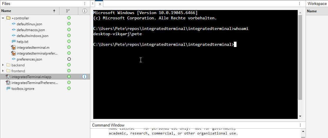
It's possible to change the shell which is used. For example, I can set the shell path to C://Git//bin//bash.exe and use Git Bash on Windows. You can also change the theme. You can run multiple terminals.
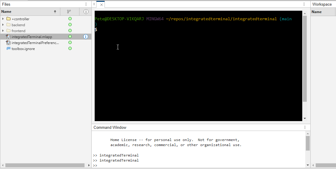
I hope you like it and any feedback will be much appreciated. As soon as it's stable enough I can release it as a toolbox.
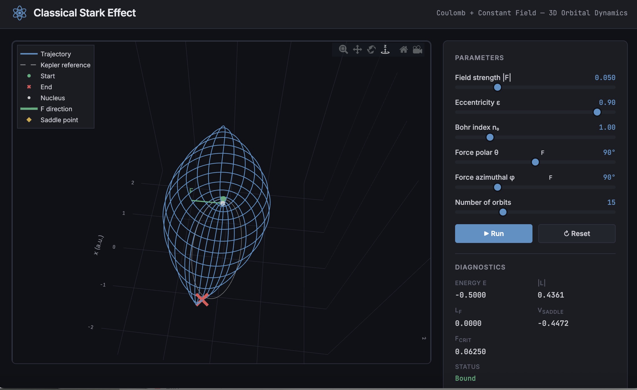
A Live Script can be converted to an HTML5 framework web application with AI as described in Double Pendulum Chaos Explorer: From HTML5 Prototype to MATLAB interactive application with AI. I have recently provides converted the Live Script Classical Stark Effect to a web application supporting a 3D twirlable display of motion of a particle subject to an inverse square law force plus an additional constant force - the problem known as the classical Stark effect.
The web application deployed to GitHub may be launched here and documents its dependencies below the interactive application. The files are available at Classical Stark Effect — Interactive Web Simulation. One gotcha was the need to enable hardware acceleration in Chrome (no problem in Safari) to support a 3D twirlable display. If hardware acceleration is disabled in Chrome, the application provides a warning and replaces the 3D twirlable display with a 2D alternate.
The conversion of the script to a web application was performed with Perplexity.ai. The GitHub deployment was accomplished with Anthropic's Claude using the open source GitHub CLI. WIth the gh CLI (already installed and authenticated on my Mac) via osascript, and Claude connected to my file system via MCP and an ngrok server, Claude executed on my Mac the following sequence of steps:
1. git init
Creates a hidden .git/ directory in the staging folder, initializing it as a local git repository. Before this command the folder is just a plain directory; after it, git can track files there. Run once per new project.
2. git branch -M main
Renames the default branch to main. Older git versions default to master; GitHub now expects main. The -M flag forces the rename even if main already exists. Must run after git init and before the first commit.
3. git add -A
Stages all files in the directory tree for the next commit. The -A flag means "all" -- new files, modified files, and deleted files are all included. This does not write anything to GitHub; it only updates git's internal index (the staging area) on your local machine.
4. git commit -m 'Initial release: Classical Stark Effect Interactive Simulation'
Takes everything in the staging area and freezes it into a permanent commit object stored in .git/. This is the snapshot that will be pushed. The -m flag provides the commit message inline. After this command, git knows exactly what files exist and what their contents are -- gh repo create --push will send exactly this snapshot.
5. gh repo create ClassicalStarkEffect --public --source=. --push
Three things happen in sequence inside this one command:
- gh repo create ClassicalStarkEffect --public -- calls the GitHub API to create a new empty public repository named ClassicalStarkEffect under the authenticated account (DuncanCarlsmith).
- --source=. -- tells gh to treat the current directory as the local git repo. It reads .git/ to find the commits and configures the remote.
- --push -- sets the new GitHub repo as origin and runs the equivalent of git push origin main, sending the commit from step 4 up to GitHub.
Without steps 1-4 having run first, --push would have nothing to send and the repo would land empty.
6. gh api repos/DuncanCarlsmith/ClassicalStarkEffect/pages --method POST -f build_type=legacy -f source[branch]=main -f 'source[path]=/'
Calls the GitHub REST API directly to enable GitHub Pages on the repo. Breaking down the flags:
- --method POST -- this is a create operation (not a read), so it uses HTTP POST.
- -f build_type=legacy -- critical flag. Tells GitHub to serve files directly from the branch. The alternative (workflow) would expect a .github/workflows/ Actions file to build and deploy the site, which doesn't exist here, and would produce a permanent 404.
- -f source[branch]=main -- serve from the main branch.
- -f 'source[path]=/' -- serve from the root of the branch (as opposed to a /docs subdirectory).
This is the API equivalent of going to Settings > Pages in the GitHub web UI and setting Branch: main, Folder: / (root), clicking Save.
7. curl -s -o /dev/null -w "%{http_code}" https://duncancarlsmith.github.io/ClassicalStarkEffect/
Not a git or gh command, but the verification step. GitHub Pages takes ~60 seconds to build after step 6. This curl fetches the live URL and prints only the HTTP status code (-w "%{http_code}"), discarding the body (-o /dev/null) and suppressing progress output (-s). 200 means live; 404 means still building.
MATLAB MCP Core Server v0.6.0 has been released onGitHub: https://github.com/matlab/matlab-mcp-core-server/releases/tag/v0.6.0
Release highlights:
- New cross-platform MCP Bundle; one-click installation in Claude Desktop
Enhancements:
- Provide structured output from check_matlab_code and additional information for MATLAB R2022b onwards
- Made project_path optional in evaluate_matlab_code tool for simpler tool calls
- Enhanced detect_matlab_toolboxes output to include product version
Bug fixes:
- Updated MCP Go SDK dependency to address CVE.
We encourage you to try this repository and provide feedback. If you encounter a technical issue or have an enhancement request, create an issue https://github.com/matlab/matlab-mcp-core-server/issues
I was reading Yann Debray's recent post on automating documentation with agentic AI and ended up spending more time than expected in the comments section. Not because of the comments themselves, but because of something small I noticed while trying to write one. There is no writing assistance of any kind before you post. You type, you submit, and whatever you wrote is live.
For a lot of people that is fine. But MATLAB Central has users from all over the world, and I have seen questions on MATLAB Answers where the technical reasoning is clearly correct but the phrasing makes it hard to follow. The person knew exactly what they meant. The platform just did not help them say it clearly.
I want to share a few ideas around this. They are not fully formed proposals but I think the direction is worth discussing, especially given how much AI tooling MathWorks has built recently.
What the platform has today
When you write a post in Discussions or an answer in MATLAB Answers, the editor gives you basic formatting options. Code blocks, some text styling, that is mostly it. The AI Chat Playground exists as a separate tool, and MATLAB Copilot landed in R2025a for the desktop. But none of that is inside the editor where people actually write community content.
Four things are missing that I think would make a real difference.
Grammar and clarity checking before you post
Not a forced rewrite. Just an optional Check My Draft button that highlights unclear sentences or anything that might trip a reader up. The user reviews it, decides what to change, then posts.
What makes this different from plugging in Grammarly is that a general-purpose tool does not know that readtable is a MATLAB function. It does not know that NaN, inf, or linspace are not errors. A MATLAB-aware checker could flag things that generic tools miss, like someone writing readTable instead of readtable in a solution post.
The llms-with-matlab package already exists on GitHub. Something like this could be built on top of it with a prompt that includes MATLAB function vocabulary as context. That is not a large lift given what is already there.
Translation support
MATLAB Central already has a Japanese-language Discussions channel. That tells you something about the community. The platform is global but most of the technical content is in English, and there is a real gap there.
Two options that would help without being intrusive:
- Write in your language, click Translate, review the English version, then post. The user is still responsible for what goes live.
- A per-post Translate button so readers can view content in a language they are more comfortable with, without changing what is stored on the platform.
A student who has the right answer to a MATLAB Answers question might not post it because they are not confident writing in English. Translation support changes that. The community gets the answer and the contributor gets the credit.
In-editor code suggestions
When someone writes a solution post they usually write the code somewhere else, test it, copy it, paste it, and format it manually. An in-editor assistant that generates a starting scaffold from a plain-text description would cut that loop down.
The key word is scaffold, not a finished answer. The label should say something like AI-generated draft, verify before posting so it is clear the person writing is still accountable. MATLAB Copilot already does something close to this inside the desktop editor. Bringing a lighter version of it into the community editor feels like a natural extension of what already exists.
A note on feasibility
These ideas are not asking for something from scratch. MathWorks already has llms-with-matlab, the MCP Core Server, and MATLAB Copilot as infrastructure. Grammar checking and translation are well-solved problems at the API level. The MATLAB-specific vocabulary awareness is the part worth investing in. None of it should be on by default. All of it should be opt-in and clearly labeled when it runs.
One more thing: diagrams in posts
Right now the only way to include a diagram in a post is to make it externally and upload an image. A lightweight drag-and-drop diagram tool inside the editor would let people show a process or structure quickly without leaving the platform. Nothing complex, just boxes and arrows. For technical explanations it is often faster to draw than to write three paragraphs.
What I am curious about
I am a Data Science student at CU Boulder and an active MATLAB user. These ideas came up while using the platform, not from a product roadmap. I do not know what is already being discussed internally at MathWorks, so it is entirely possible some of this is in progress.
Has anyone else run into the same friction points when writing on MATLAB Central? And for anyone at MathWorks who works on the community platform, is the editor something that gets investment alongside the product tools?
Happy to hear where I am wrong on the feasibility side too.
AI assisted with grammar and framing. All ideas and editorial decisions are my own.