Draw Images from a Picture or Webcam | Arduino Engineering Kit: The Drawing Robot, Part 3
From the series: Arduino Engineering Kit: The Drawing Robot
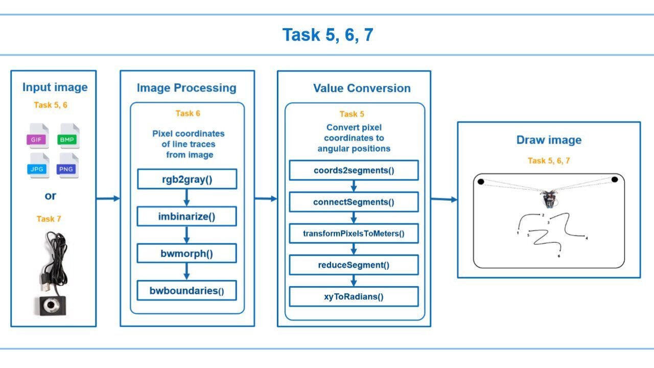
In part 3, learn how to process an image from a file or a webcam and convert it into motor commands to perform the drawing motion of the robot. See tasks 5-7 of the Arduino Engineering Kit. These tasks implement the algorithms to convert the input image into motor commands. Specifically, the input image transforms into pixel coordinates, which subsequently converts to angular positions of the motors.
Published: 2 Sep 2021
Hi there. Welcome to the final video of this video series. Now that you know how to move the robot to a particular location, and also know the accessible regions of the whiteboard, we are ready to move one step forward where we will draw an image on the whiteboard.
We are going to look Task 5, 6 and 7. The schematic of the same is shown in this slide. As you can see in Task 5 and 6, we will input a saved image. Whereas in Task 7, we'll input the image captured from a webcam. In Task 5, we will first convert the pixel coordinates to the angular position. Here, we were already given the pixel coordinates. Once done, in Task 6 we will closely look at how we can get the pixel coordinates of the line traces from an image.
Finally, in Task 7, we will repeat all the steps and Tasks 5 and 6 by inputting an image captured from a webcam. Let's get started with Task 5. First, we'll load an image in MATLAB. We have already provided you the coordinates of pixels from the image that describe the line traces of that image. Later, in Task 6, we will look at how we can get these pixel coordinates from an image. But for now, let's use the provided coordinates.
The coordinates are stored in the cell array named segmentsPix. This cell array contains two columns with each row corresponding to a single pixel coordinate. To visualize different segments stored in segmentsPix variable, you can plot them by running the plot pixels chosen from sample image section. As you can see in the image, different segments are drawn in different colors.
By now, you might have noticed that the coordinates represent the line traces of the image that we want to draw. Note the actual line traces on the whiteboard, but you won't have a marker to follow. Thus, we will have to convert the data from pixels to meters. To do this, we have provided you with the function transform pixels to meters. This function allows you to specify the percentage of available space you would like to use to draw the image.
Feel free to open and dig inside the function file if you want to know how it works. Let's now plot the segments defined in meters. You can see the plot looks the same as before except for the units. If you look closer, you will see that the points to be drawn are very close to each other and in larger numbers. To save some time, let's filter out the segments to reduce that net drawing time.
We can do so by specifying the minimum distance between two consecutive points, and then can remove all the points from the segments such that they all are at least that far apart. Let's again plot the line traces, but now with the filter reduced points. Now you should see the fewer points which can reduce the time to print the image significantly.
Next, we will input the initial position and then use the route optimization function to optimize the drawing path to reduce the drawing time further. Just like we did earlier, we will then use the xy to radians function to convert the target position in meters to target angular displacement of the motor shaft. Once we complete these steps, we can connect the hardware as done before.
Now we are all set to draw an image on the whiteboard. To do the same, we will read each line trace in a loop and extract the target angler position values of the motor shaft. Then we will move the robot to the first position, lower the marker, move the robot to all the positions in the line trace, and then finally raise the marker. We will repeat these steps for each line trace in the image.
Whoohoo. I'm sure you must be thrilled to draw your first image. Let's now understand the workflow we use to extract the line traces from the image in Task 6. Start by loading an image using the imread function. Then we will process the image such that it will only contain the thin traces of the line. In this process, we will convert the image to grayscale, convert it to binary black and white, remove isolated pixels, and then thin out objects to lines.
Once you have the thin line image, you can use the pre-built function getCoords which will generate a sequential list of pixels from the preprocessed image. Next, we'll call coords2segments function which will segment all extracted pixel coordinates into the different segments. This step can give us some segments whose end points are adjacent.
We will now call connectSegments function to reduce the total number of segments in the image. This function merges any segments whose endpoints are adjacent and closes any segments that intersect themselves. In the previous exercise, we needed the minimum and maximum pixel values for the processed image to scale the pixel values to meters. Using the pixel coordinates, we will compute the same to use them later by drawing the image.
To make things look cleaner, we have encapsulated all the above steps into a single function called imageToPixelSegments. Similar to what we did in the previous exercise, we can hang our robot on the whiteboard, measure initial string lengths, and use the pre-implemented function to draw the image on the whiteboard. Wonderful. You have successfully built your drawing robot. Give yourself a pat on the back.
Just one more thing before we wrap up. So far, you have been working with a saved image that you clicked some time back. But how about drawing a live image that your webcam captured just now? This is what we will do in the next exercise. We will first click an image using a webcam. Then, we will ask our robot to recreate the same image on the whiteboard.
First, connect the webcam provided in the kit to your computer, execute the connect to webcam section to connect MATLAB with the webcam, then join the preview webcam image section to view the live feed from the webcam. You can now capture any drawing you would like your robot to recreate by executing the captured the current image section.
To ensure that the captured image will be drawn correctly by the robot, you can call the imageToPixelSegmens function and check the traces for their accuracy. If the processed image seems a little bit off, try to capture a new image. After you are satisfied with the captured image, you can go back to the previous exercise and input your captured image to draw it on the whiteboard.
Hooray. You have done it. You have built your own drawing robot using Arduino Engineering Kit. Now you are free to go wild and try out some of your own images. Thank you for watching this video series.

Featured Product
MATLAB


Select a Web Site
Choose a web site to get translated content where available and see local events and offers. Based on your location, we recommend that you select: United States.
You can also select a web site from the following list
Americas
- América Latina (Español)
- Canada (English)
- United States (English)
Europe
- Belgium (English)
- Denmark (English)
- Deutschland (Deutsch)
- España (Español)
- Finland (English)
- France (Français)
- Ireland (English)
- Italia (Italiano)
- Luxembourg (English)
- Netherlands (English)
- Norway (English)
- Österreich (Deutsch)
- Portugal (English)
- Sweden (English)
- Switzerland
- United Kingdom (English)