Change for the Better: Improving Predictions by Automating Drift Detection

[MUSIC PLAYING]

Hello Peter.

Hi can you hear me?

Yes, perfectly well.

OK

Welcome

We're ready?

We are ready.

Hello

OK, I'll get started then. OK, thanks everybody, for coming today. Today we're going to talk to you about how to automate a predictive maintenance application for a fleet of electric vehicles. I know the title of this talk is Automating Drift Detection. But we've actually automated most of the process, as you'll soon see.

Before we get started, I want it to be very explicit about what I hope you'll remember from today's talk, an understanding of the kinds of machine learning problems our method can automate, how to build a production system that operates with minimal human supervision, and the key technologies required to construct such a system. Today we're going to demonstrate how we built a predictive maintenance applications for a fleet of electric vehicles.

As the world moves toward carbon neutral technologies, electric batteries are showing up in very diverse places, city buses, farming machinery, and factory floor automation. Machine learning powered predictive maintenance enables us to manage these batteries more effectively than simply replacing them according to manufacturer guidelines. We're going to focus on that bus.

Let's imagine a Metropolitan Transit system wants to use machine learning to manage their fleet of electric buses. They want to know when a bus battery needs maintenance or replacement, before it fails and strands the bus full of passengers. If they have a monitoring system in place, the vehicle can send a notification of the failure to a dashboard. Then they'll definitely know they need to replace the battery.

But that's not really an ideal solution. What they'd really like to know is when the failure will occur, to move from monitoring to prediction. They've hired a couple of engineers, us, to help them build a solution.

So here's what we propose, a system that uses sensor data from the batteries to predict when those batteries will fail. Here's how it works. As a bus moves through its day, the battery cycles through various levels of charge. And onboard instrumentation sends the battery state data, like current and voltage, to our application. And that's where our machine learning model transforms the raw data into knowledge they can use, a prediction of the battery's state of health, allowing them to schedule maintenance and allocate resources to keep the buses running on time.

But none of this is really new. Predictive maintenance solutions like this have been in use for several years. They perform well. But they are complicated and require a lot of human intervention. And that won't work for this client.

Our bus company doesn't have much AI expertise. So it's very important that the solution requires little post-deployment maintenance. How will they know if a proposal meets that requirement?

Machine learning operations, or ML Ops, illustrates the process of continuous integration and deployment with this diagram. The left hand loop focuses on the deployment, the development and training of the model and the right hand loop on the model's performance in production. In order to satisfy the low maintenance requirement, the solution must automate, as much as possible, of both of these loops.

Automation of some parts of the ML Ops cycle is well understood. Deployment and operations, for example, usually run autonomously. But closing a loop requires monitoring and evaluating model performance and then sending feedback to the development arc.

And that's where a deep understanding of the problem domain is so important. The system must incorporate that feedback into a better performing version of the model. And then the new model can be sent into production.

It's important to realize that not every machine learning problem can be automated like this. To understand which ones can, let's take a high level look at the monitoring, feedback, and training technologies in our solution for the bus company. One way to know if you need to retrain your model is by analyzing the data your model is processing.

Drift detection analyzes the difference between a training set and the observed data. If the difference is significant-- in ways that Gokhan will explain in more detail-- the model no longer reflects the real world and retraining is necessary. And then the retrain model needs to be redeployed, of course.

But in order to retrain the machine learning model on the drifting data, we need to label the observed data, which usually requires human supervision. In this case, however, we have a superpower. And this is it. A physical model of the battery that simulates battery behavior accurately enough to label observe data with the battery state of health.

This model was developed with Simulink and enables us to capture physical processes so precisely that we don't need to experiment with an actual battery. We feed in sensor data. And the simulation can tell us exactly what those readings would mean for a real battery state of health.

It's accurate enough that we can use the labeled data to train our machine learning model. And we couldn't build our solution without it, because it operates without supervision. If you're wondering why we don't just deploy this physical model instead of our machine learning model, hold on to that question, because Gokhan has got an answer for you.

And speaking of retraining, AutoML enables automatic retraining by searching for a machine learning model that outperforms the current model on the original training set and the new drifting data. AutoML operates in a feedback loop. Training data enters the system, models are tuned in compared until the best one emerges and is integrated into the rest of the system.

So that's the three technologies we used, drift detection, physics-based labeling, and AutoML, to allow us to build this solution. And with that, I'll turn things over to Gokhan who will tell you how these three techniques actually work.

Thank you, Peter. Before delving into the details of the data-driven solution that we, as engineers, have cooked up for the fictional Metropolitan Transit system. Let us remind ourselves what the solution looks like.

You may remember these building blocks from Peter's talk earlier and how they mapped the infinity diagram that embodies the ML Ops framework. We can simplify this diagram to end up with this schematic. My talk will revolve around the blueprint of the system presented on this slide. We will walk through and elaborate on each piece of the cycle.

That said, there's one element that's missing from this blueprint. And that is the data piece. Every machine learning problem starts with data. High quality, accurate data is key for the success of any machine learning project. The problem at hand is also a machine learning problem. It is the problem of predicting state of health for the fleet of electric vehicles owned by the Metropolitan Transit system.

In an ideal scenario, the first step in this project would be for the company to collect data from the batteries of their fleet of vehicles, before even attempting to tackle the machine learning part. As you may have guessed, Metropolitan Transit system does not exist. Thus there is no fleet of electric vehicles nor do we have access to their data.

Fortunately, we do have access to a simulation environment. To be able to generate data, we create the physics-based simulation for the battery systems of electric vehicles using tools such as Simulink and Simscape. The simulations incorporate dynamics from different physical domains, such as electrical and thermal. This allows us to generate realistic data sets.

We also simulate the fleet of vehicles by using multiple models with different parameters. In this project, we simulate the battery systems for 20 or so different electric vehicles, using our physics-based simulation models. For each vehicle, we measure the current jump from each battery, the voltage across the battery, and the state of charge for the battery, which is the level of charge of the battery relative to its capacity.

The raw data that we measure from our models are time series data. We extract features from this data by processing it in frames with the fixed frame rate. Remember the cycle from before. The collection block, which would plug into the cycle, is thus replaced by data generation block in this project. Indeed, it moderates all the other parts of our solution.

In this project, we use simulation models to mimic real data. But one can imagine, real companies using simulation models at different stages of their solution. Data collection, in general, is costly. Thus, such models can act as digital twins for data generation as a preliminary step to data collection, to validate the behavior of the algorithms, providing a cost effective validation solution at early ages, early stages of machine learning projects.

Let us now focus on other pieces of this puzzle. Remember that the motivation behind our solution is to automate the whole process. To that end, we also need to be able to automate the model selection and training part, if possible.

This leads us to one of the building blocks of our solution, which we colloquially referred to as AutoML. This block automates the training aspect of the machine learning system. AutoML's job is to automatically find a machine learning model and hyper-parameters for this model to optimize a desired metric, while maintaining generalization. Thus, the task of finding the right model is delegated to the AutoML solution.

Let us have a bird's eye view of how AutoML operates. Starting with the training data, AutoML first selects a machine learning algorithm, say, a regression support vector machine. Using an optimization scheme, such as a Bayesian optimization, or a synchronous successive helbing algorithm, it finds the optimal set of hyper-parameters for the given model, which in turn optimizes the desired metric.

For our problem, you may consider this metric to be the cross validation means squared error. This also should tell you that our model is indeed the regression model, regression problem. This is done for other models and other hyper-parameter options, until the best model and the set of hyper-parameters are determined.

We already mentioned regression support vector machines. Models that are trained using AutoML include linear regression models, Gaussian process models, ensembles of boosted decision trees, random forests, and fully connected feedforward neural networks. It is important to point out that this optimization is done over the joint space of models and hyper-parameters of models. Thus, model selection itself is also a hyper-parameter, in this process.

Here's a short snippet of the AutoML process in action. As can be seen from this animation, the AutoML process loops through different models and hyper-parameter options, and selects the models and hyper-parameter options so as to minimize the desired metric. Note that this animation is from a classification problem. But the same idea applies to our problem and regression problems in general.

When AutoML is done training, it will return a single machine learning algorithm that we can deploy to the production server and use for prediction.

Up until now our AutoML solution has been operating under the assumption that the data which it trained does not change. Indeed, in most machine learning problems, there's an implicit assumption that the data used for changing the model fully represents the underlying distribution of the whole feature space. In other words, it is assumed that the distribution of the data does not change.

In the aforementioned problem of predicting the state of health for the electric vehicle batteries, this assumption would imply that we can collect data from several different vehicles, train a regression model, deploy this model onto all the other vehicles, and safely use this model for prediction. Unfortunately, this assumption rarely holds in the real world. Real world training data will, in all likelihood, not represent the whole distribution of the data in the feature space.

Consider the following plausible, albeit exaggerated, scenario. Imagine that during the development of our algorithm, we only had access to data from the electric vehicles operating in Europe. For the sake of the argument, imagine that the temperature for the collected data has the following distribution.

If we're not careful about the fact that our assumptions do not hold everywhere in the world, we may naively want to use this algorithm for the vehicles operating in say, Addis Ababa in summer, where the temperature distribution may be vastly different or in Siberia, say, Novosibirsk in winter, where the temperature distribution is, again, very different, from both the rest of Europe and Addis Ababa. In this case, the algorithm developed under static data assumption will most likely not work well in other parts of the world. It is thus desirable to detect changes in the data, developing over time or across regions, and react, most likely, in the form of training new models.

This change in the data is referred to as drift. In machine learning drift, or commonly referred to as concept drift, is formally defined as the change in the joint probability of observed features and labels or responses over time. Using this definition, it is quite challenging to assess concept drift for machine learning models that are used in production, because we would need to know both the features and the ground truth labels or responses, in order to be able to do this.

Getting ground truth values for responses in a reasonable amount of time for models in production may not be feasible. Thus, we can do the next best thing. We can look at changes in the distribution for what we can observe, the features. We call this type of drift, data drift or feature drift.

The idea is to collect observed data for some time and compare values in the new data, the target data, to the baseline data, which is, in our case, the data used for training our algorithm. To achieve this, we use a drift monitoring system. In our automated solution, the drift monitoring system periodically compares the distributions of the features in the baseline data to the distributions of the features in the recently observed target data. If the distributions are indeed different, it raises a flag.

Using the drift monitoring system, we can gain insight about each features' drift status and severity. In our drift monitoring solution, we estimate the likelihood of existence of drift for each feature using statistical approaches. We consider, for each feature, the null hypothesis that the observations in baseline and target data are coming from the same distribution. And we test this null hypothesis separately for each feature in our data.

Then, given the significance, level we estimate how likely it is for us to see the vectors that we are observing in the target data, assuming that the null hypothesis holds. We also estimate the confidence intervals for our estimations. For instance, in this plot, we can see that for a feature, say, the signal to noise ratio for current, under the null hypothesis, the probability of observations for this feature in target data coming from the same distribution as the observations in the baseline data is estimated to be about 25%.

With a significance level of 1%, we fail to reject this null hypothesis and conclude that we do not see any evidence of drift. As long as we are certain that the estimated probability and the confidence interval around it is completely outside of the drift and warning thresholds-- which are 1% and 5% in this specific plot-- we may cut off our estimation early and do not analyze further, and make an early decision. This is indeed what's happening for this specific feature.

Note that the drift monitoring system operates in an automated way as well. But the monitoring system can also alert the supervisor. In the case of such an alert, the supervisor can look at plots, such as the ones we just saw, in more detail and make the decision to override the system if desired. Thus, our drift monitoring system allows for human supervision as well.

There's a crucial question to be asked here. Does data drift automatically imply that our model is outdated and needs to be retrained? The answer is no.

We cannot say, based on the output of the drift monitor alone, that the model is not performing well, because we can't know if our model's performance is degrading, unless we have the ground truth values for responses. Which in, our case, is the state of health for the batteries. What we can do is, we can assess if the data distribution has changed. And if it did, we can then request the labels for the data in order to assess model performance.

Remember from our previous slide that we use the word react and not act, in the presence of drift. This is because we don't necessarily want to keep training new models with every incoming batch of data. This would be very costly. We want to do this only when the model's performance is indeed affected by drift.

Our drift monitor allows us to do just that. When it raises a flag, we propagate the drifting data through our model-based labeling system, to automatically label the data. Note that our machine learning problem is not a classification problem. It's a regression problem. However, for the sake of having a generic module name, we simply refer to this module as the model labeling system.

In our solution, we use a high fidelity model-based labeling system implemented in Simulink. We propagate recorded observations through this system and estimate the ground truth response values, which are the state of health values for the batteries, by simulating the model dynamics. You may be asking why we're using a machine learning based system to predict the state of health, if we can estimate them with the simulation model in the first place. The reason for using a machine learning based predictor is because we require near real time response times from our predictor. And the model-based labeling system's simply not fast enough to achieve this response time.

In our solution, we utilize the simulation model to label observed data only when it is prompted. This happens when the drift monitoring system sends an alert signaling data drift. It is important to understand that, even though this idea of model-based labeling works for our problem, it may not work for all other data-driven solutions. That being said, our framework is flexible enough to allow for a different labeling system, where the labeling task may be completed by different means, for instance, by crowd sourcing, subject experts, or by other means, maybe even with the aid of another machine learning model.

Once the labeling is complete, we look at the model's performance on the label data. If the drift indeed results in model performance degradation, we go back to retraining and challenge your model. Using our AutoML solution, a challenger model is trained with the augmented data that is composed of both the original training data and the new data, and performance is compared to that of the champion model, the model in production. If the challenger model performs better, the challenger would replace the model in production, thus becoming the new champion.

So this is it. This is the automated machine learning solution we have created for the Metropolitan Transit system. It is composed of several modules that are responsible for automated training and retraining of machine learning models, prediction using deployed models, drift monitoring, and automated labeling of data using simulation models.

Our solution implements the cycle of training, deployment, monitoring, and labeling. And it works automatically for each vehicle in the fleet. And it ensures that each vehicle's inference model gets updated whenever the model performance degrades.

Last but not the least, we envision an automated system implemented this cycle. But it's flexible and modular enough to allow for other workflows that require closer human supervision. And with that, I'd like to end my section. And I'd like to pass the microphone back to Peter.

Thanks Gokhan, my goal for the last part of this presentation is to show you how to build an automated machine learning system for yourself. I'm going to do that by walking through our implementation. I'll highlight some of the challenges we faced, and how we overcame them, and describe what we needed from our development environment.

Each of the four phases that Gokhan described maps to a concrete module in our system. Since we've automated the entire ML Ops cycle, the system can react to change without requiring time consuming human intervention. Now we'll walk around that loop, following the data as it flows from raw messages to actionable knowledge.

And as we've moved from the abstract to the concrete, I'll also mention the additional components we need to create our working system. A streaming service, like Kafka, handles the data coming in from our fleet batteries. The machine learning model loads from the model registry and then makes a prediction. It also saves the observed data for drift detection and labeling.

Periodically, the drift detector examines the input data. When it detects drift, it notifies the labeler to create new training data from the observed data. In our case, the drift detector also publishes drift data details to the streaming service for downstream display.

Once the labeler has created the new training set, it notifies the AutoML Retraining System, which evaluates multiple models in parallel, using the original and the new training set data. A champion model emerges and uploads to the model registry for distribution to the predictors. And all the while, there's a graphical dashboard reading their predictions and drift data, and generating a display for the maintenance crew.

We built very little infrastructure ourselves. Because our solution consists of so many off-the-shelf components, we were able to focus on algorithm development. And as for the components themselves, we got sensor data streaming into Kafka, MATLAB Production Server hosting prediction and drift detection.

We built the physical battery model in Simulink. MATLAB drove the AutoML retraining, using MATLAB Parallel Server to train the model in parallel. We had Redis for our model registry, and InfluxDB as our time series database, and Grafana as the framework for our dashboard.

Now you've seen the overall architecture, I want to focus on how we transform that diagram into a practical system. First, I'll highlight three challenges that drove the architecture. And then, I'll identify the characteristics of a development environment, suitable for building and automated machine learning solution.

Our biggest challenges were data order and frame size, machine learning model distribution, and horizontal scaling. And our must-have development environment features are a virtual production environment, native access to streaming data, and deployable physical models.

Recall what Gokhan told you about feature extraction. It's accurate only if the frame contains a minimum number of messages, all from the same battery. But since multiple buses send data to the stream simultaneously and independently, messages in the stream seldom present themselves in suitable blocks.

Note there's two problems here. Not enough data from a single battery to fill up the frame, four in the stream but the frame needs six. And all the messages are not in a contiguous block. Since the frame-- wait, hang on a second.

So first we grouped the messages in the stream into a contiguous blocks by battery. Then we pick a battery and send all of its messages into a frame. Since the frame isn't full, the predictor returns without making a prediction.

Eventually, more messages from the same battery appear in the stream and are transferred to the frame. Since the frame is full, the predictor consumes the messages and makes a prediction. And we build parallel frames like this, simultaneously, for all the batteries that have appeared in the stream.

Because the predictor returns instead of waits, we're not under utilizing our hardware resources. There are multiple predictors. And each one has access to all the partial frames. So as soon as one frame fills up for any battery, we emit a prediction. And that's as fast as we could go, as fast as the messages arrive from the stream.

But that scheme only works if we can actually have multiple predictors operating simultaneously. And that raises a subtle challenge. How do we prevent multiple predictors from making a prediction for the same battery?

To answer that, we look to the streaming service. To support simultaneous operations, the streaming service places the streaming data into one or more partitions. Each partition may be read or written simultaneously.

Fortunately, well by design actually, the streaming infrastructure provides two guarantees. All the data for a given battery will stream from the same partition. No two predictors will be called with data from the same partition. And those two combine to ensure that no two predictors ever operate on data from the same battery, at the same time.

I'd like to make one last point about the architecture, before moving on to a discussion of the development environment. Having a single repository for the model allows the AutoML process to publish the model to a central location. And then each predictor can fetch new models when it's ready.

The model registry maintains one model per battery. Since a given predictor may work on data from any given battery, it's hard to predict which models each predictor will need. This pub/sub architecture allows predictors to ask for models as needed and simplifies model development.

Now I'd like to transition to an overview of the features you should look for when selecting a development environment to help you automate the ML Ops cycle. So now I'm going to demonstrate what I mean by-- I'm going to show you a demo of the development environment first. And then we'll walk through the features.

And I'm going to demonstrate what I mean by stream integration and a virtual production environment. This is MATLAB. Let me start the video.

And here's how you create a stream object, in this case a connection to Kafka. And here's how you read from that stream, turning events in the stream into a timetable. To start the virtual production environment, you first bring up the server. And then you start streaming data to it asynchronously.

Oh, hang on. What happened there? So let's just run that again. Once that's running, you can monitor the requests here to see how code will react in production. Let's put a break point in the prediction function. We're still monitoring that here.

Now we can debug and test as we ordinarily would. Here's a prediction, for example. And here's the values of the features that we're predicting with. The server's paused until we let it go. And when we're done, we can stop.

So now that you've seen what the development environment looks like in action, I want to talk a little bit more about each of the pieces. Data scientists understand how to develop a predictive maintenance model using historical data stored in files. Read data, load the model. Make a prediction. Write it to the file and save the model if it change.

That's a very familiar and productive paradigm. We found it very useful to have a development environment that allowed us to replace files with streams, because it's easy to go from one to the other. We could easily move from processing historical or synthetic data to live production data, without having to change our code.

So what does interactive access to streaming data look like in practice? Let's start with what an event looks like on the streaming server. This is one raw message stored in JSON in Kafka. The event payload is pretty simple. Eight variables and their values stored as key value pairs.

Most of the values appear to be floating point numbers. But notably, the key, or battery ID, is an integer. Associated with each message as a schema, which describes the data properties of the payload.

The format is pretty verbose, so I'm only showing a description of the current variable, which the schema asserts is a scalar double with a default value of zero. That's data package for transport, not algorithm development. And you don't want to have to manually convert it to something your algorithms can process.

Since this is a time series data, we'd like a timetable. I'm only showing the first four columns here. But that's enough for you to see that the timetable current is a double, just as the schema specifies.

And here's the code that produced the timetable. One line to create a stream object, just like you'd open a file, and then a second to read from the stream. The stream object applies the schema to the streaming data automatically.

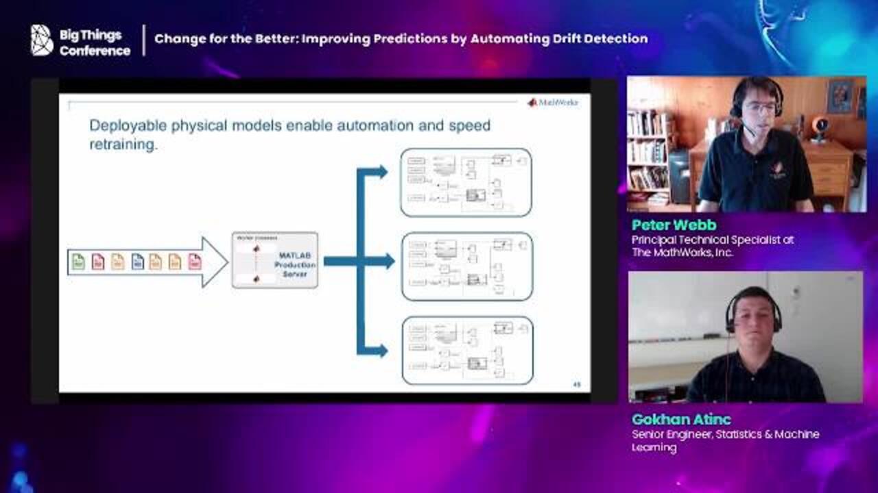
So the last important development environment feature involves a different kind of model and a different kind of transformation. Physical model simulation environments are often a kind of import-only ecosystem. You can bring in data from the outside world. But you can't run the models outside of their interactive desktop application.

But if you package your models so they can, well, then they start to behave like machine-learning models and algorithms. If you host them on a server, they'll scale. You can spawn as many of them as you need to handle the incoming stream of data. Since our labeling process is like our predictors, battery specific, we can safely operate as many labeling models as there are batteries, if we really need that kind of performance.

Don't let this make you think we're replacing the machine learning prediction algorithm with the physical model. That's not our intent at all even scaled like this, the model is too slow to provide the performance we need. We're deploying this physical model in order to automate the ML Ops cycle. Deployed like this, it can run autonomously without requiring human interaction. And that's what we wanted in a development environment, a virtual production environment, native access to streaming data, and deployable physical models.

And that wraps up the architecture section of the talk. Now I'm just going to give you a short video of the whole system in action. I don't have time to step through the whole system. But I can show you some of the highlights.

First, here's a script that automates the process. It starts by predicting the original model, then runs drift detection on the observed data and retrains the model. That's once around a loop. Then it predicts, using whatever model emerged from the training process and looks for drift again, and so on.

Let's take a look at how retraining works. Here's the output from the end of the retraining stage. You can see two of the candidate models and some of the statistics used to evaluate them. And at the bottom, we're told that none of the newly trained models performed better than the original. So the champion retains the crown.

What does this mean for the predictions? Let's take a look at the dashboard. We trained the original model with 20 batteries and used it to predict the health of five, as the number in the upper left indicates. 40% of the 5 in our fleet are apparently experiencing drift. But all seem to be in relatively good health.

Let's take a look at the battery with the most drifting features. Battery 10 has six drifting features and declining health. Though the two are not necessarily related. If we compare drifting and a non drifting that is stable feature, it becomes clear how important the algorithms are.

Can you tell these two apart? I know I can't. And as for our first round of retraining, let's see what effect that had. Not much, as we should expect. You see nothing changed, since the original model beat all the challengers.

But in the third generation, one of the challengers won. And you can see that the predictions have tightened up. And we're still detecting drift in the battery.

So that's it, sensor data all the way from the buses via Kafka, through MATLAB's machine learning algorithms and production servers, and into a Grafana-based dashboard. I hope this gives you some idea of what you can do with these tools.

There's enormous opportunity in the complete automation of the ML Ops cycle. If you reduce the need for people to manage parts of the process that are tedious, error prone, and frustrating, you'll free your data scientists to focus on what they're best at, creating solutions. And that truly is a change for the better. So thanks very much.

[MUSIC PLAYING]