Why Padé Approximations Are Great! | Control Systems in Practice
From the series: Control Systems in Practice
Brian Douglas
Watch an introduction to Padé approximations. Learn what Padé approximations are and how to calculate them, why they are important, and when to use them—specifically in the context of time delay and control system design.
Published: 13 Jun 2022
In this video, I want to introduce you to Pade approximations. And we're going to cover what a Pade approximation is and how to calculate one. But what I'd really like for you to take away from this video is why they are important and when to use them, specifically in the context of control system design. So I hope you stick around for it. I'm Brian, and welcome to a MATLAB Tech Talk.
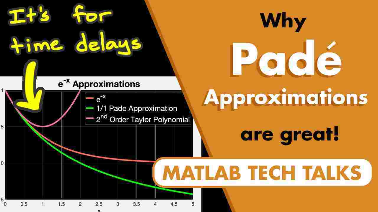
As the name suggests, a Pade approximation is an approximation of a function. And the idea is that we take any function and approximate it as a rational polynomial. So for example, let's take the function e to the minus x, which I've plotted here. The first order over first order Pade approximation for e to the minus x is 1 minus 1/2 x over 1 plus 1/2 x. And if I plot this, you can see that it approximates e to the minus x pretty well up to about x equals 0.5 or so.
Now instead of a first order over first order, we could also choose higher orders like a 2 over 2 Pade approximation. And we can see that the higher order approximation does a slightly better job of matching the original function. Now these are just two examples. And in general, we can choose a Pade approximation with any numerator order and any denominator order.
For example, this table shows the Pade approximations for e to the minus x up to order 3 for both the numerator and the denominator. So there are an infinite number of Pade approximations for a given function. And generally speaking, the higher the order of the rational function, the better the representation becomes.
So this is what a Pade approximation is. It's a rational polynomial or a ratio of two polynomials of any order that approximates another function. So why is this important? I mean, what's the point of using an approximation when we can just use the original function?
Well, one of the main reasons why I use Pade approximations is for representing time delay in dynamical models of systems. To show you what I mean, let's walk through a simple example. This is a spring mass damper system. And the input u of t is a force applied at the mass.
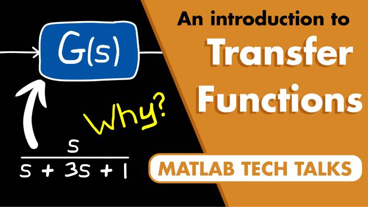
And the output y of t is the position of the mass that we measure with a sensor. And assuming that there's no delay in the system, then the transfer function from the input force to the output position is 1 over Ms squared plus bs plus k. Or for the parameters of our system, it would be 1 over S squared plus 0.5s plus 1.
So now let's go over and create this transfer function in MATLAB using the tf command. And then we'll plot the step response. So what does this show us?
Well, the step command applied a force of 1 newton at time equals 0 seconds. And then this plot shows the position of the mass over time. And we can see that the mass started moving right at 0 seconds and then ultimately was offset by a distance of 1 meter. But the important thing that I want to point out is that the measured position of the mass starts to move the instant force is applied. There is no delay in this model.
However, let's assume that the real sensor actually has some delay. Maybe it takes an entire second for the sensor to calculate and output a measurement. And if we want to incorporate this delay in our model, we can do so with a transfer function. The Laplace transform of a time delay is e to the minus s tau where tau is the length of the delay in seconds. So a 1 second delay would be e to the minus s.
And in MATLAB, I can add a delay when I create the transfer function. And as expected, our model is now e to the minus s times the original transfer function. And now if we take the step response of this system, the response is the same shape.
But it's delayed by 1 second. We don't sense that the mass is moving until 1 second after the force is applied due to the delay in the sensor. And being able to capture a delay like this in a model is really important for accurate simulations, and for system analysis, and for controller design.
I mean, for example, let's assess whether a unity feedback controller produces a stable closed-loop system. And at first, let's start with our model that doesn't capture the delay and then plot the open loop frequency response using a Bode plot. With this plot, we can look at the stability margins. And it looks like we have infinite gain margin and about 41 degrees of phase margin. And so it's saying that our closed-loop system is stable.
Well, at least our model without delay is claiming that it is. However, if we look at the Bode plot for the system with delay, which more closely matches the real system, we see that the delay adds additional phase lag, which lowers the frequency response curve and impacts the stability margins. And, importantly, we can see that our stability margins are now negative and that the closed-loop system is actually unstable with this delay. So at least in this example, it's important to account for delay in our model. Without it, we might be deceived into thinking our design is sufficient when it actually isn't.
And, fortunately, there are a lot of tools that can handle delay in this exact form, the e to the minus s tau form. I mean, we just saw that Bode plots work perfectly fine with time delay. And this is because delay just adds all of that additional phase lag to the system, which can be displayed and interpreted easily in the phase plot.
However, there are some tools that don't work with time delays. For example, root locus doesn't work. If we plot a root locus for the model without delay, we can see that it is a plot of how the closed-loop poles move from the open-loop poles to the open-loop zeros as the loop gain increases.
And the problem is that a continuous time delay is essentially an infinite number of poles. So it's going to be difficult to display all of those lines on a graph. In fact, if I try to plot a root locus in MATLAB for the model with delay, it throws an error saying that it cannot be used for continuous time models with delays and to use the Pade approximation instead.
But root locus isn't alone time delay doesn't work well for other control methods either like LQR or H-infinity synthesis. Again, it's this infinite number of states problem. If you're doing full state feedback like LQR, then you need to feed back an infinite number of states. Or in the case of H-infinity, you'd end up with an infinite state controller. And neither of which are practical solutions.
So like the MATLAB error says, this is where Pade approximation comes in. We can replace the exact function e to the minus s tau with an approximation in the form of a rational polynomial. Or since the variable is the Laplace variable s, then this turns out to just be a rational transfer function. Essentially, we're capturing the essential dynamics of the time delay in a continuous time transfer function that now has a finite number of states.
So with that behind us, let's look at how we can actually calculate a Pade approximation of e to the minus s tau. And there are several different methods. But the one that I want to walk through in this video is actually by calculating a Taylor series first. The Taylor series for e to the negative x at x equals 0 is the summation from n equals 0 to infinity of negative x to the n divided by n factorial, which can be expanded to 1 minus x plus x squared over 2 minus x cubed over 6 and so on.
Now to convert this into a Pade approximation, we first need to decide the order of the rational polynomial that we want. Remember this Pade approximation table? Well, basically, we need to pick a numerator order m and a denominator order n. And for this example, I'm going to choose a first order for both. So we're going to calculate this result here.
A Pade approximation of order m over n is this rational function R of x. And it might look intimidating. But if I expand this for order 1 over 1, we get this much simpler a0 plus a1x divided by 1 plus b1x.
And now we just need to figure out the coefficients a0, a1, and b1. And we do this by equating it to the Taylor polynomial of order m plus n. And since both the numerator and denominator are order one, then we would equate this rational polynomial to a second order Taylor polynomial. And now we just solve for the coefficients.
So to solve this, we multiply both sides by the denominator. And then we get this equation. And then to solve for the coefficients, we can look at each of the x terms individually.
So we'll start with x to the 0. So, basically, we're looking for terms without any x's in them. And on the left side, we have a0. And on the right side, we have 1. So a0 equals 1.
Now we move on to x raised to the power of 1. And on the left side, we have a1. And on the right side, we have negative 1 plus b1. So there's not enough information just yet to solve for a1 and b1. But let's move on to x squared.
On the left side, we have 0. And on the right side, we have 1/2 minus b1. And so this makes b1 equal to 1/2. And then if we use this in the equation above, we can solve for a1 equals negative 1/2.
And at this point, we've solved for all of the coefficients. But we still have a leftover term in the equation. That's this x cubed term. So what do we do with this?
Well, it just gets ignored. Remember, we only need to consider up to second order terms. And so the x cubed term is discarded during this process. And ignoring this term actually makes the Pade approximation different from the Taylor polynomial. And it kind of seems like magic.
But by solving this equality and then discarding the higher order terms, we've produced an approximation that's a better fit of e to the minus x than the second order Taylor polynomial. And it kind of makes sense if you think about these results as transfer functions. I mean, given the same number of states, a transfer function with poles and zeros can produce a more complex behavior than one with just zeros.
All right, so we did this calculation with order m equals 1 and n equals 1. But we could do this method for higher orders as well. And so with that being said, two questions come to mind.
One, how do we determine which order Pade to use? And, two, why are we limiting ourselves to equal order polynomials for both the numerator and the denominator? I mean, when we showed this table earlier, we can see that there's all sorts of mixed order polynomials. So why are we so concerned with 1 over 1 or 2 over 2 or 3 over 3? Well, let's actually start with that question.
Each of these are approximations of e to the negative x. And we could choose any of them to represent it. However, only the equal order Pade approximations-- those are these along the diagonal.
Only these produce an approximation that affects only phase and not gain. They act like an all pass filter. And to see what I mean, let me plot the 2 over 2 Pade approximation and compare it to the 2 over 3 approximation.
Notice that with the 2 over 2 the gain is 0 decibels for all frequencies. And it's just the phase that is affected by this system. Whereas with the 2 over 3 approximation, the gain starts to fall off at higher frequencies. And since a time delay doesn't affect gain in any way, it just delays the signal and therefore just the phase, this all-pass type of filter is preferred.
So we typically try to limit the Pade approximation to equal order polynomials for both the numerator and denominator. But now let's address the first question. Which order do we choose? And the answer comes down to the amount of delay and the speed of the system. And to understand that, let's look at the Bode plot for e to the minus s plus the first few orders of the Pade approximation.
And notice that as the order of the approximation increases the phase matches the real function to a higher frequency. The 2 over 2 approximation is good up to about 2 radians per second or so. The 3 over 3 is good to about 4 radians per second. The 4 over 4 is good to about 6 radians per second and so on.
And so we can choose the order of the approximation based on which frequencies we care about in our system. And if we're designing a closed-loop controller, often this comes down to the cutoff frequency or the frequency at which the gain drops below negative 3 decibels.
As an example, we can go back to the spring mass damper model that we developed earlier and look at the Bode plot for the transfer function with delay. The open-loop cutoff frequency of this system is about 1.5 radians per second. So if we wanted to replace the e to the negative s term with an approximation using poles and zeros, we'd want to make sure that the phase is relatively similar, at least up until this frequency.
And for a 1 second delay, we know that a 2 over 2 Pade approximation would fit the bill. So our rational transfer function that takes into account the essential dynamics of the time delay would look like this. And now instead of limiting ourselves to loop shaping a controller with a Bode plot, we could use this new model and look at the root locus or do full state feedback and LQR or any other technique that requires a rational transfer function or state space representation.
All right, so this is where I'm going to leave this video on Pade approximation. If you don't want to miss any other future Tech Talk videos, don't forget to subscribe to this channel. And if you want to check out my channel, Control System Lectures, I cover more control theory topics there as well. Thanks for watching, and I'll see you next time.
Related Products
Learn More


Select a Web Site
Choose a web site to get translated content where available and see local events and offers. Based on your location, we recommend that you select: United States.
You can also select a web site from the following list
Americas
- América Latina (Español)
- Canada (English)
- United States (English)
Europe
- Belgium (English)
- Denmark (English)
- Deutschland (Deutsch)
- España (Español)
- Finland (English)
- France (Français)
- Ireland (English)
- Italia (Italiano)
- Luxembourg (English)
- Netherlands (English)
- Norway (English)
- Österreich (Deutsch)
- Portugal (English)
- Sweden (English)
- Switzerland
- United Kingdom (English)