Data Preprocessing for Finance
Sourcing, cleaning, and preprocessing data is a challenge. Learn how to spend more time building models and less time cleaning data using MATLAB®.
Published: 11 Oct 2020
Hello and welcome to today's session on data pre-processing with MATLAB. Prior to beginning today's session, let me introduce myself. I'm Lawrence. I joined MathWorks in January 2020. Prior to joining MathWorks, I used to work as a quantitative developer for an index provider. As part of my role, I used to collect data, process it, and construct indices for customers based on their requirements.
Something that I've found true myself is the 80-20 principal. I'm sure anybody who works with data has experienced this firsthand. You spend 80% of their time cleaning data, finding data, aggregating data, and 20% of the time fitting models and deriving useful insights from your data. Although there is value to spending 80% of time working with data, you can spend a lot more time getting insights from the data if you could automate a lot of the data pre-processing and cleaning tasks. For this kind of automation, MATLAB is the ideal environment. And our objective today is to see some ways in which MATLAB simplifies the data pre-processing task.
Here's the agenda for today. We'll start off by looking at typical challenges people face while handling data.
After that we have four demos. The first one is a valuation example of fundamental data. We take some stock data, which has issues like outliers, missing data, stock splits, and we will see how we can resolve these issues using MATLAB.
The demo after that, which is about cleaning the large data sets. Imagine you have 50 GB of data and your computer has just 4 GB of RAM. How do you work with these kind of data? Logically, you would split them into chunks and this is how you would work with it. But instead of you doing it, MATLAB has something called tolerance, which does this for you.
The next demo is data cleaning by machine learning, where we fit a small machine learning algorithm to predict the value that are missing in our data set. And the last demo is the text analytics example, where we look at the SEC filing of Apple and we derive insights from it without actually having to read the document.
In the end, we open the floor to your questions.
Let's start off with some typical challenges in data management. There are three major challenges. The first of these is the large amount of data sources, the storage type, the different format, and different technologies that go along with it. The second one is poor data quality, and the third one is the need for customized analytics.
Let's have a look at the first challenge when it comes to data cleaning and management. We're starting to see a lot of data coming in from a variety of sources. A couple of years ago, data was mostly text or numericological. Nowadays we have alternative data, such as satellite images, audio signals, weather data, you name it, you can find data for it. As diverse as it may seem, the storage of data is just as diverse. A couple of years ago we used to work with databases, flag files, Excel files. Nowadays you have the possibility to store your data in Spark Hadoop clusters. You can scrape web pages.
While we used to work with table data and panel data in finance a couple of years ago, we're starting to see a trend towards working with text data or a sentiment analysis of tweets, sentiment analysis of-- we're starting to see more trend towards text analytics.
The next challenge is the poor data quality. So as you can see here, on the left hand side, I have a CSV file where in the first column I have security ID and then some quarterly information. For the first three rows, you can see that I have a lot of missing values. And this is part of the example that we will see today. Here I have the Apple EPS data, and I see one outlier. I have some missing data here as well.
The next challenge is the need for customized analytics. With the onset of alternative data providers such as Quandl, RavenPack, and others, analysts are looking for edge with finding more data and more unique data. This implies there is no one size that fits for all users of data.
Right. With that, let's start having a look at the demo that we have set up for today. The first one is the fundamental valuation example.
So the goal is to rank stocks based on the historical EPS trends. The approach is simple. We access data from CSV files, we pre-process them to clean up the text, missing data, outliers, and then we calculate the strength of historical EPS trends.
Right. So with that, let's just jump to MATLAB. So for those who are unfamiliar with MATLAB, that's what MATLAB looks like. On the left hand side, you have the current folder. Here you have the command window, which is basically a giant calculator. You can set values to variables, you can add, you can multiply. It just becomes a giant calculator. So if you had noticed, for each of these commands over here, MATLAB was keeping a memory of whatever variable or command we typed in over here in workspace. So this is kind of the memory of MATLAB.
To clear the memory of MATLAB, type in Clear, and that text takes away the variables from workspace. And to clear the command window, I type in CLC. Right.
Prior to starting the demo, let's have a look at the Excel file that we're working towards. So here we see a relatively clean Excel file. You have the symbol, you have the date for standard security ID, the name of the stock, industry. Here are the EPS values that you've calculated, the sentiment. Now based on this data, I've created a pivot table over here, aggregating stocks based on their industry and then calculating the average EPS trend measure for the industry.
Let's have a look at how we can do all this using MATLAB. So prior to starting the exercise, let's have a look at the data. We are going to be working with three different Excel files. One is the ticker data. So you have the stock symbol and you have the security IT.
The next one is-- whoops, let's close that. [INAUDIBLE] on this outside MATLAB. You have the security ID, you have the name of the company, and you have the sector information.
And then the last file that we will be working with is the earnings per share diluted quarterly data.
So here you have the security ID and you have the quarterly information from the first quarter of 2011 until the second quarter of 2017. You have the security ID and you have some missing values. We'll see how we can work with this. So let's go ahead and close all this.
Let's go back to where we were. So we're going to be working on something called the live script. To create a live script it's simple. You start by clicking this button over here. What live script does is you can combine text, formatted text, code, and the output of the code along with it.
So, for example, I've got this bit over here, which is text, and this is the code. To execute this code I can either press Control and Enter, or I could just go ahead and click this blue bar over here.
Let's start with what we were going to do. So over here, I have this function, import company data, for reading in the CSV file. Have a look at it, you can see that this file has been auto-generated by MATLAB. How do we get to that place? So for doing that, all I have to do is double click on an Excel file or CSV file. MATLAB proposes how it would be read into MATLAB.
So, for example, if I want to import the selection over here, it imported ticker S&P 100 as a table. I could bring these up as column vectors, as numeric vectors, string array, or cell array. And we can also instruct MATLAB on what to do when it finds unimportable cells. At this point, you could just import the selection or you could say generate function. And then it generates a function similar to what we saw earlier.
And this is particularly useful, because let's say you close MATLAB and you start the next day and you have the same starting setup. Instead of importing the variables again, you could just use that function, which we have over here.
So let's start by importing our data into MATLAB. So here I have companies. The information I have over here is the security ID, the name, and the industry. One thing to note over here is the number of lines that we have. We have roughly 12,600 stocks. In the next instance, we are importing S&P 100 ticker data. So here we are looking at the stocks within the S&P 100 [INAUDIBLE].
And just for your information, this function has been generated the same way we saw earlier. So if I look in here, this has been auto-generated by MATLAB. Although it has been auto-generated, you can see that it is using couple of functions, lower level functions, which MATLAB uses to read these files. You could either treat these as black boxes, or you could use these functions that MATLAB generated to learn how data is read into MATLAB.
So here we have read in the tickers data. So we have the symbol, we have the data for [INAUDIBLE], and we have the security ID. Now we're going to be joining these two tables, companies and tickers based on the stock security ID. So for joining this, it's similar to joining two sets in mathematics. You have the inner join where you pick up the intersection of the two data, [INAUDIBLE] join where you pick up the entire data set, left [INAUDIBLE] join where you pick up the data from the left table.
So for doing this, you have this cool feature called live tasks, where you can join tables. And this is how you insert the live task for joining tables. In my case, I've configured how to configure the table. So let's have a look at that.
I'm instructing MATLAB you join the data and store it into a variable called ticker data. My left variable is tickers, left table is tickers, and the merging variable is [INAUDIBLE]. My right table is companies and my merging variable is SEC ID. I can choose to see either just the control or just the code or both the control and the code. And I can do that by having a look over here.
Let's execute that. So here you see that it has merged these two tables. So we had 102 rows over here. We had 12,604 rows away here. On merging, we have 12,606. So this means there were two extra lines in our new file over here.
OK. So we are starting to see a lot of missing symbols. So the symbol information was coming from the S&P 100, but just 102 stocks had symbols. OK, let's clean this bit. Let's have a look at the date first added attribute of the S&P 100 data. OK. So we're seeing stocks that have been added until the end of 2014, 2015, roughly. OK. So let's filter for missing data and let's take out all the missing data. Now to have a look at data, I could either hover over the variable this way. So you can see a lot of [INAUDIBLE] have been taken out. Or I could do head of ticker data.
Now let's import the quarterly earnings per share data. So here you can see I have my security ID and I have my quarter information. Keep in mind that I don't have the date over here. I just have Q1, Q2, Q3, for 26 quarters. OK. Now let's just keep only-- once again, one thing to note over here. We have roughly 11,000 stocks over here. Let's just keep the stocks that are in the S&P 100 universe.
So now if I hover over my data variable, you can see that it's roughly 60 stocks that have been filtered down to, and I have security ID for them, and I have the quarterly information for these stocks.
Now let's go ahead and replace these Q1, Q2, Q3 with actual dates and then transpose these columns to rows, thereby helping us to create a new kind of data called time table. Let's go ahead and do that. So if we were to find the quarterly dates for end of quarter, from beginning of 2011, that's the command line date shift from beginning of 2011. We're finding the ending of quarters and we need 26 such quarters. So we get 31 March, 2011 until the second quarter of 2017. Let's go ahead and transpose the table and then convert that table into a time table.
So here you can see that dates column have been grayed out as well. This means that it's a time table, as MATLAB has indicated over here. So the advantage over here is that you can index into each of these roles using dates. And here you have the stocks as columns. Here we are plotting three of these stocks to see what [INAUDIBLE]. So here we see the histograms and here we see the scatter plots.
Now if, as I pointed out earlier, I could hover over the data or open the data by saying open data, and here you can see the keyboard combination for opening data is Control plus D. Let's open this data.
So here you can see there are a couple of negative values for 30th of September, 2015, AIG had a negative value. 31st of March, 2016, it had a negative value. Same case for Target. So let's go to our live script and get rid of these negative values. What I'm doing is wherever there are negative values, I'm setting them to not a number. Now let's open data.
So now you can see that I don't have negative values, but instead I have NaN. I'm actually going to be filling in these NaN values. Let's go ahead and look at what the NaN values look like. So here we have some NaN values at the beginning, a few in the middle, and some of these stocks have no NaN values or little NaN values, and some of these stocks have just NaN values.
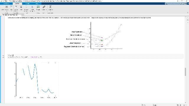
OK, so we'll see how we can actually treat this kind of data. OK, so for completing the missing data, There are several algorithms that you could have. For example, here in this data, we saw this image earlier. We have a couple of missing data here. And we could choose to interpolate this data. There are several algorithms that MATLAB provides for you. So mean substitution, you could substitute the mean, median, or regression.
It really depends on what kind of data you're working with. If you're looking at price data, you probably want to forward fill the last available price. If you're working with stock attributes you probably want to interplay the data.
So for doing that, again, you have one live task over here for cleaning missing data. And that's how you insert it. Let's get rid of that. So here I am instructing MATLAB to store the cleaned data into this variable called clean data. The data table that I'm working on is data and here's the variable that I need cleaned. The cleaning method I specified as clean interpolation.
One feature to keep in mind is this green dot over here. What this tells MATLAB is as soon as I make some changes, I want it to go ahead and calculate. So I can actually switch it off or leave it on. So let's go ahead and do the computation. And you can see how MATLAB has filled in these values. These orange points are the filled missing entries.
If I go ahead and choose line interpolation, you can see how it has filled in. And you could see that MATLAB completed the calculation as soon as I chose this algorithm. If you do not want it to happen, if your data is too big and you think that it is slow-- I mean, it is taking time every time you do this, you could switch it off, make the changes, and do the computation like so.
So let's go ahead and fill the missing value. Now if I go ahead and look at data, you can see that most of the NaN values have been replaced. You see that it has been replaced. On the other hand, we saw some where we did not have any values to work with. So these stocks, we're going to simply remove them.
So let's go ahead and do that. [INAUDIBLE] missing. So now at this point we go back and look at our data we do not have any stocks which has NaNs.
Let's go ahead and start by looking at outliers. So this is our stock, this is the box plot, and each of these red cross shows us that there is an outlier in the data. OK. For cleaning outliers, once again, you have a live task over here, clean outlier data. You can insert it by clicking this button. In my case, I have already laid it out. I'm instructing MATLAB to store these clean data into this variable over here. The table that I'm working with is data, and the variable that I'm working with is ABT. Let's go ahead and execute that.
So here I've instructed MATLAB to clip outliers at this threshold factor. I could also choose to fill in the nearest value, in which case, you see what's going on. [INAUDIBLE] the previous value, for that matter. And in this case let's stick to clipping the threshold value.
OK. Now let's go ahead and see what that does to our data. So here in this box plot, you can see you no longer have these red crosses and your data is relatively-- your data does not have outliers. Let's go ahead and apply that to our entire data set.
In the next case, we're looking at a 7 for 1 stock split. We've been told that there has been a 7 for 1 stock split in June 2014 for the Apple stock. So if we look at it, you can see that there is an upward trend for this stock and then a sudden decline and then continuing upward trend. So we are told that this is the point where this split has occurred. Let's try and see if MATLAB can programmatically identify where that switch has happened.
So if we're doing that, we are looking at a live task, which can identify change points, this one over here. So let's go ahead and execute this live task. So here you can see that MATLAB has correctly identified where the change has happened. So it has put this green vertical line and defined the change point. What we're doing is we are looking at the change of mean and the maximum value of the first-- the highest change of mean value. If we increase the points, we would see more drastic changes of mean, but in our case, the first one is the one that we're looking for.
Now let's correct for that. Let's have a look at the date when this happened. So we identified that it happened on the 30th of June, 2014. Now let's adjust for the EPS after stocks split [INAUDIBLE]. So what we're doing over here is creating a time range from the date split until today. And for all that data in that time range we multiply it by 7. And then when we have a look at it, we see that it's a continuously upward trending data.
All right. In the next step, the fitting a curve on our data and thus identifying the trend measure. We are fitting a curve on the EPS data. We fit this curve and we get the trend measure, which is a proxy for our EPS data. And then we sort the stocks similar to what we saw in the Excel file, by the EPS data. So here we are looking at the top 10 rows using the top [INAUDIBLE] command. Here we specify the top 10 rows. Over here, we can see we have the top 10 stocks sorted based on their trend measure. Here we see a lot of the same as well.
In the next step, we're going to create something we did in the Excel file using the pivot table. We aggregate the stocks based within the industry by calculating the mean of the trend measure of each stock within the industry. So here we have a table that resembles what we saw in the Excel file. And with that, we come to the end of the first demo.
Let's go back to the presentation and have a look at what we saw. So together, we saw how we use interactive tools to import and visualize data. We generated code by-- we automated by-- we made MATLAB write code on its own, and we built in cleanup functions as well. We were able to align and calculate group statistics. And by doing all that we were able to save a lot of time.
All right. With that, let's go to the next demo, which is about cleaning large data sets. The objective is to calculate technical indicators on big intraday data. The data that we have obtained is by scraping data from the web. We will probably look at missing data, outliers, and we will actually clean this data. The approach that we take is pretty simple. And it is similar to what we saw earlier. We pre-process the data, we explore the data, and then we calculate the technical data.
So we alluded to this earlier, tall arrays. What are they? So in order to work with tall arrays, you need something called data store. What this does is it points to the location of the data. In our case, you could see this [INAUDIBLE] over here. It's a lot of CSV files. We are telling MATLAB that our data is located in CSV files, and a lot of them, and here's where you find that data.
Once you have identified the data scope, you create the tall array. Oh, just one thing that I forgot. Your data store could even point to databases or even Spark Hadoop clusters. Now once you have defined your data store, you define a tall array by calling the tall function on your data store. What this function does is to tell MATLAB that if the data were to be present in MATLAB, if the data were imported into MATLAB, this is what it would look like. It would look like a tall array.
Once you have defined the tall array, you can operate on this tall arrays as you would on any other array in MATLAB. You would use the same functionality. So what tall array does is it breaks up data into small chunks that fit into memory. And then it scans through one chunk at a time.
The way you process tall arrays is the same as ordinary arrays. If you have Parallel Computing Toolbox, you can process several chunks simultaneously. And it scales well with MATLAB Parallel Cluster. And let's go ahead and go into the demo. So we are done with this. Let's close this.
So prior to going into the live script, let's have a look at what the data looks like. So here you can see we have a couple of CSV files from 28th of July until the 17th of August. And what do they look like? So you have date, close, high, low, open, volume, and you have minute-wise data, so 9:30, 9:31, 9:32, until 4:00 PM of a given day. So that's roughly 392 lines per CSV file. OK. We'll see how we can work with this kind of data in MATLAB.
So let's go ahead and create a datastore as we saw earlier. So you can see that we just specified the kind of data that should come in, is in [INAUDIBLE]. We have this specified as white [INAUDIBLE], and it has correctly identified all the files that has to come in. It has identified the variable names, the structure, and here we have a preview of the data store.
Let's import a subset of the data. We import a subset using read command. If you want to bring in the entire data into MATLAB, you would use the command Read All, which reads in the entire data set. In Read, you're looking at a certain number of lines which you have specified in your data store.
If I open my data store, you would see the read size, which is 20,000. In our case, the first Excel file has 392 lines. And that's what it does right into this subset, 391. So here I am plotting the close prices on the right hand side and the volume prices on the left hand side.
Now let's go ahead and create a table array, tall array. So here, it is asking MATLAB to switch on the parallel [INAUDIBLE]. So it is setting up for parallel computing. And after creating the tall array, we are telling MATLAB to create a time table out of the stable data.
So here we are connected to the parallel [INAUDIBLE]. Now let's have a look at what the table looks like. So here you can see you have a small subset and something curious over here. You have a couple of dots. At this point, MATLAB just knows that this is a tall time table, and if the details are entirely imported into MATLAB, this is what it would look like. At this point, we can go ahead and continue working with this tall array the way we would in any other area on MATLAB.
So let's have a look at the tall array. Here you can see a bunch of question marks. So this is similar to having your data within MATLAB, but you don't actually have it. So let's think of an analogy. Let's think of an array that you have in each box, the formula that tells MATLAB what the value of that cell would be. So think of this cell containing the formula that brings in the value in the cell. And we do not have that value populated. So that's what we are working on.
In addition to that, if you want to actually create visualizations on this tall data, MATLAB does it in runtime. So it plots the tall data, and when you zoom into that particular part of the tall data, MATLAB actually reads the data in real time and then plots it.
So here you can see that it has actually plotted the data, the tall data from the beginning of-- from the first CSV file until the last CSV file. And here we see the minute wise data as well. We see the volume data shows a lot of fluctuation. And here we are computing the data for the third plot. That said, at this point you could go ahead and zoom in and MATLAB would compute the data again for where it needs to zoom in. So this is done in real time.
At this point, we're going to do a lot of calculations. And the result of the calculation, we cannot actually see it right now, because if you hover over these variables, you can see that it is telling MATLAB that the formula-- that the way you should compute this variable is by using this function over here. But do not just compute it yet. We will do it at the end using a function called Gather.
So here again, we are doing the same thing. We are telling MATLAB that these are the variables that you need to compute, but do not just compute it yet. These are the functions which you should work with. Here's the moving average, daily moving average of the volume weighted average price. Again, we see question marks. Here I am synchronizing the tables. And once again you can see there are question marks. Here I am computing the intraday volatility, the rolling volatility, the range of the volatility.
And at this point, you can see that you have a lot of values which have been set up. A lot of variables, which have been set up with calculations but without the actual values. In this next step, we're using this function to gather the value of each of these into-- gather the value of each of these variables using the formula that have been set for it. Let's go ahead and do that.
So here you can see that MATLAB has split the data into chunks and it is working on each of these chunks in parallel. So what MATLAB is doing over here exactly is what you saw in the presentation. So we started off by setting the data store, where we told MATLAB that we have all this CSV files. Then we created a tall array to tell MATLAB if the data were to come in MATLAB, this is what it would look like. And then we worked on a couple of functions to work on the data.
And at this point, when we called Gather, MATLAB started working with that data one chunk at a time. It scans through the data set one chunk at a time, which fits in the memory. And it is doing all that function, the calculation that we saw earlier for each of these variables. When you have Parallel Computing Toolbox, it does this process in parallel.
Let's go back to MATLAB. So that's what is being done over here. It is computing in parallel each of these variables.
It has to go to two more of these passes, and we are done pretty soon.
OK. So at this point, you have the values for each of these variables which have been calculated. So if I look at my first variable, you see that instead of question marks I have the values computed. You can see that I no longer have question marks. Instead I have the values that I was actually looking for. So it has computed all these variables. Now I can go ahead and visualize the data that I just computed.
Right. Now that brings us to the end of the second demo.
So what have we seen over here? Here's the summary. We worked with big data, just like that, in our memory, and we broke down the data into small chunks without actually having to go through MapReduce or other big data technologies. We saw the visualization of big data was easy as well. We were not using any different functions. We were using just the same more functions that we use in MATLAB. MATLAB does the heavy lifting of identifying what the data is and plotting the data. And we saw how scalable that MATLAB model is.
With that, let's go into the third demo, which is data cleaning by machine learning. This is relatively a small demo. We won't go into the weeds of the algorithm, since MATLAB 101, which is part of these presentation modules. What we're going to look at is filling the data by random forest algorithm.
So first off, we start by importing data. So here we see we have our price information, we have a couple of missing coupon data, yield to maturity, current yield, and some information on if it is callable or not. Let's have a look at the summary data. Here we see the number of missing data to be seven, in coupon we have nine missing values, in yield to maturity we have five, you get the idea. We have a couple of missing values.
Now we have a user-defined function called [INAUDIBLE], which fits a random forest on our data and then it predicts the missing value. So let's go ahead and do that.
So here it's failing in the data based on the machine learning algorithm. Let's go ahead and look at the output data. So we saw a couple of NaN values over here, not a number values here. We do not see any missing values over here. And we can see that they kind of make sense over here, these data. Now let's have a look at if we have any missing data. We have no missing values here, none here, none here, no missing values. That's good. That's the end of the third demo.
Let's go ahead and look at the fourth and the final demo, which is the SEC filing. So the import data that we're working with, the SEC filing, if we look at it as the typical kind of data that companies provide to SEC, it's a PDF file. And we'll be working with it. So here's the live script that works with it. And the output that we are working towards is to get insights from this PDF. And here we start with the first sentence and here we have the last sentence. And we're looking at how important each of these topics are from the beginning towards the end.
So just to have an idea, in the beginning, you talk a lot about your partner, supplier risk, and somewhere in the middle, and towards the end as well. And the bigger dot implies that higher probability of its appearance in being in the text. So we'll have a look at that.
Let's start by bringing the PDF file into MATLAB. So here we see that it has brought in the entire text into MATLAB. In the next step, we are splitting between the section 1A and section 1B and we are reading all the item between-- in section 1A, which are risk factors.
If I look at my string, I could still have some kind of links, which do not give a lot of information to me. So let's go ahead and clear that. At this point, you can see that I have converted my string to this, the cleanup data. And now let's go ahead and visualize the most frequent words in our data.
For that we use word cloud, which plots the most frequent word. So in our data we're using, we are seeing a lot of the word company repeated a lot of times. And the exact count of it, you can find in this table over here.
In the next instance, we are splitting these sentences into documents. So we have identified in the first sentence, we have nine different tokens. Token is how many different words we have in a sentence. In the next sentence, we are looking at what are some trigger words, like, do we have the word supplier? Are there some suppliers that could possibly depress the stock? So we're looking at that in our cleaned documents.
But despite the fact that we have done this, do the words like and, is, in, add value to us? In our case, no. So we are removing it using these functions over here, remove short words and remove empty words.
The next step, we are going to compute the sentiment of our SEC filing. A sentiment of 1 indicates the sentiment associated with this document is positive. A sentiment of negative 1 indicates the sentiment associated with this document is negative. A score of 0 indicates a neutral statement. In our case, it's slightly positive, it means that it's slightly neutral, positive document that we have.
Now let's fit the Dirichlet model and identify the topics that we have in our SEC filing. So here, by looking at the different word bubble, we can see that there are four major topics. One is the partner supplier risk, the manufacturing operational risk, the economic risks, and the legal risks. Let's go ahead and have a look at how important each of these topics are. See that these are roughly of same importance. And let's go and have a look at the importance of each of these documents from the beginning of the document towards the end of the document.
So here you can see on the x-axis, this is the starting sentence and this is the final sentence. And here's the probability of each of these topics. Here we are looking at different kinds of-- here we're looking at the way the importance of this topic evolves throughout the document.
And there you go. That brings us to the end of the demo. So we have seen how, using MATLAB, you could process your data faster and get to building insights a lot faster. Just in this last example, you've got to identify what are the important topics and how the importance evolves without actually having to read through the PDF document.
And at this point, I am open to taking your questions.
Featured Product
MATLAB
Up Next:

Related Videos:


Select a Web Site
Choose a web site to get translated content where available and see local events and offers. Based on your location, we recommend that you select: United States.
You can also select a web site from the following list
Americas
- América Latina (Español)
- Canada (English)
- United States (English)
Europe
- Belgium (English)
- Denmark (English)
- Deutschland (Deutsch)
- España (Español)
- Finland (English)
- France (Français)
- Ireland (English)
- Italia (Italiano)
- Luxembourg (English)
- Netherlands (English)
- Norway (English)
- Österreich (Deutsch)
- Portugal (English)
- Sweden (English)
- Switzerland
- United Kingdom (English)