Control Design Tasks | Design and Test a Grid-Tied Solar Inverter Controller, Part 3
From the series: Design and Test a Grid-Tied Solar Inverter Controller
Learn how to leverage a full system model to explore the design of different control modes for a grid-tied solar inverter. Control design tasks and analysis that are covered include how to,
- Select appropriate model fidelity
- Tune PID gains automatically
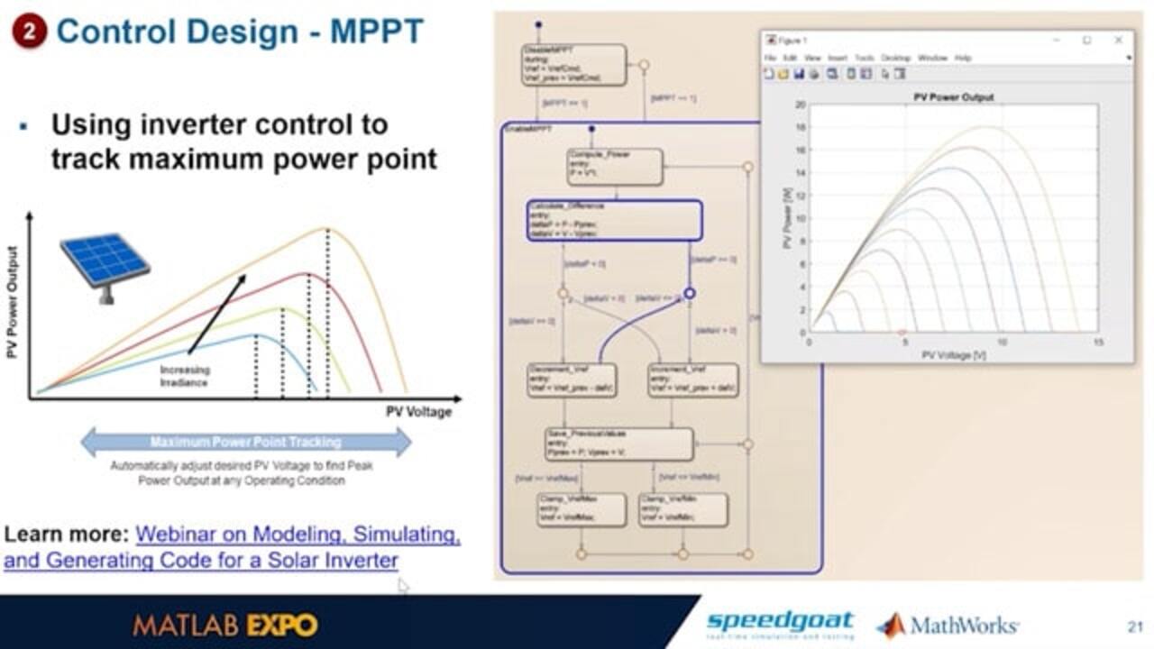
- Develop a Maximum Power Point Tracking (MPPT) algorithm
- Assess Fault Ride-Through
- Assess against Grid Codes such as IEEE 1547-2018
Published: 6 Jul 2022
So now that we have a model of our power inverter, what we can do is we can start to leverage that for design tasks such as control tuning. Now one of the most important things that we need to do when we're building an inverter that connects to the grid is to actually control the control loops that we have here.
So we have current loops and we have voltage loops for solar inverters. One of the most important loops is our voltage regulator. That's actually going to allow us to control the power output of the photovoltaic system.
Now, for example, in this case we want to tune this DC voltage regulator. But we have power electronics.
One of the advantages of building a model, especially using our Simscape electrical tool, is we have average-value models in approximations for most of our common inverter topology bridges. And this will allow us to extract a linear-transfer function out of this model very easily and go jump right into control tuning so that we can identify good control gains for the performance that we need.
So, for example, if we were to look at the system here, our solar inverter system, jump into our inverter control. Right now we have our DC voltage regulator with some gains to start. If we run a simulation of this, we can look at the performance of this voltage regulator in terms of the whole system.
Now, going inside of this PI controller, we could take a look. We could adjust these gains by hand. That's very good. But we can also use our auto-tuning methods. Now this is going to grab that approximation that we have of this model, given the average value approximation that we have. Grab that linear transfer function and allow us to directly start to do PID tuning.
Now what this process looks like, is once we've got that transfer function for our solar inverter and the grid connection, we can start to do tuning. And so in this case, we're tuning it for one operating point. But we could do the same process for multiple operating points if we wanted to do something more like a gain schedule controller.
For voltage regulators on solar inverters, that's typically not necessary. If we're happy with this performance, we can then send these new updated gains back to the PI controller and start to do full simulations. And so we've updated our gains, we can rerun the simulation here with the new improved performance to see how this improved voltage regulator performs.
And in this case, we do a voltage step and we see much faster performance. So we talked here about this voltage regulator. Right now, we've been applying just voltage steps, DC steps. But in an actual system, we'd be looking more at our maximum PowerPoint tracking algorithm.
This is an algorithm that's going to seek out the maximum PowerPoint of an inverter given-- or of our solar array, given different operating conditions. And so that's going to be, actually, what's going to dictate that voltage reference step.
And so, typically, to implement this you want to basically create an algorithm that can seek the maximum power output of the converter-- of the solar array, given basically irradiance on the panels, and then also the loading situations on the inverter.
There's many types of methods for maximum PowerPoint tracking. In this case, we're using a perturbent-observed type of method where we're basically incrementing our voltage reference and observing what's the power output. And then if it's not high enough, we can start to increase it or decrease it, accordingly.
And we could see, as it kind of did that, it always was seeking out the maximum point, either on this irradiance curve, or if we had a lower irradiance, it was trying to find this peak here.
And, finally, we've been talking about kind of the low-level controls. On top of that, we have this idea of this being a grid-connected system. And so we can also look at our performance as a grid-tied system here, especially when faults occur.
And so, using the same stateflow-based state machine logic, we can come up with a routine basically goes through islanded performance. It transitions into grid connected. And then when a voltage fault happens, you'll see that the voltage drops here. We can transition to reactive power support during that fault and adhere to grid codes, as we talked about in the beginning.
Now looking at grid codes, these are things that we can test in Simulink, as well, on both simulation and then also in hardware in the loop. And so there are many different grid codes out there. One of the most common ones for renewable energy is 1547. There has been a 2018 revision for that.
And we can kind of replay events through our models and see how our system performs and if we disconnected or not. And we've produced a block for this. And you can kind of replay and see how the system performs. And if you exceed the threshold and disconnect before you should, we could flag that and say this would not adhere to 1547 or other good codes, for example.
We have a webinar on this material if you would like to learn more.
All right. Now starting to tie this all together, we have kind of the high-level controls, the DC voltage regulator we talked about, and we have the system model. So we can run this full simulation to kind of exercise all these different control scenarios to see what our performance is before we target hardware.
One of the most important things is being able to synchronize with the grid before we actually connect. And so we can see that our control systems are able to do synchronization using phase lock loop.
And then we can kind of see, once we do connect with the grid, how much active and reactive power are reproducing in this case. And, by default, the controls are going to emphasize active power response. And we should see that here in a second. At 10 seconds we're going to close the breaker to connect to the grid.
And we can see now that the three-phase current in this case, the electromagnetic transience occurs. And we can see both the voltage and the current wave forms in this case.
Now, right now, we're assuming there's a constant irradiance. We can adjust the irradiance. We could feed in a profile or just change this manually to take a look at different values. You can see as we drop the irradiance our active power output decreases.
Of course, this is tying together with the maximum PowerPoint tracking algorithm, which is still seeking that maximum power output point.
Related Products
Learn More


Select a Web Site
Choose a web site to get translated content where available and see local events and offers. Based on your location, we recommend that you select: United States.
You can also select a web site from the following list
Americas
- América Latina (Español)
- Canada (English)
- United States (English)
Europe
- Belgium (English)
- Denmark (English)
- Deutschland (Deutsch)
- España (Español)
- Finland (English)
- France (Français)
- Ireland (English)
- Italia (Italiano)
- Luxembourg (English)
- Netherlands (English)
- Norway (English)
- Österreich (Deutsch)
- Portugal (English)
- Sweden (English)
- Switzerland
- United Kingdom (English)