Developing Field-Oriented Control Algorithms for Brushless Motors
Overview
Field-oriented control is a popular means of controlling brushless motors used in automotive, industrial, aerospace, and consumer applications. Motor Control Blockset for Simulink speeds up the development of a field-oriented controller by helping you to verify control algorithms using simulation and generate compact and efficient code for a microcontroller.
In this session, MathWorks engineers will walk you through a reference example of field-oriented control algorithm simulation and code deployment to a TI C2000 microcontroller for a permanent magnet synchronous motor (PMSM).
Highlights
- Model motor and inverter dynamics at different levels of fidelity
- Design a field-oriented controller, including current, and torque/speed loops using a quadrature encoder or Hall sensor
- Implement Park and Clarke transforms, and a space vector generator
- Use automatic PID tuning to set the controller gains for current and speed loops
- Verify controller performance through closed-loop simulations
- Generate code for a Texas Instruments C2000 microcontroller and operate the current loop of the PMSM at 20 kHz
About the Presenters
Anton Vesenmaier
Anton Vesenmaier is an Application Engineer at MathWorks. His main areas of expertise are automatic code generation for embedded systems and AUTOSAR, systems engineering and other tasks in the context of Simulink.
Eva Pelster
Eva Pelster is a Senior Application Engineer at MathWorks. She holds degree in Aerospace Engineering from the University of Stuttgart. Her focus at MathWorks is on model-based design workflows and physical modeling applications.
Recorded: 24 Nov 2021
Hello, and welcome to today's webinar. My name is Anton Vesenmaier. I'm an application engineer at MathWorks and together with my colleague, Eva Pelster, we are going to talk about developing field-oriented control algorithms for brushless motors.
Hello, and welcome.
Eva, can you briefly show our viewers and me what we will see in today's webinar?
Sure, Anton. So today, we will use the example of a brushless motor and look into how model-based design can support you in making a motor spin. So we will see how the algorithm can be developed and simulated in Simulink, and how that same model can then be reused to generate embedded code.
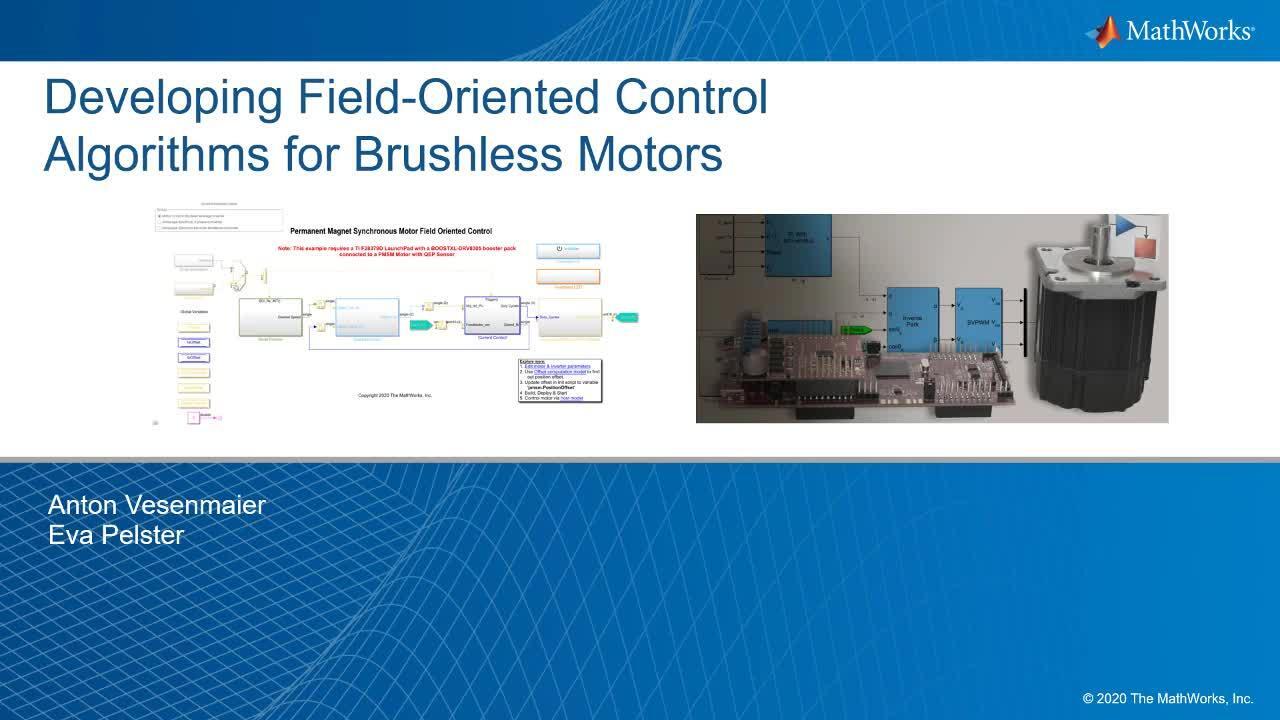
So here we can see a quick first glance at the model. The algorithm is already implemented. And by making use of automatic code generation, we can directly deploy the algorithm to our hardware setup up, making the motor spin, and we can also use Simulink as an interface to change the speed input commands.
So this layouts a typical workflow, parts of which we will look at today. We will start by calibrating the sensors, and using the captured data to estimate motor parameters, then creating a model of motor and inverter, and based on the achieved model, we can then design a control algorithm, and deploy and validate on a final environment. The errors within the workflow indicate the iterative nature of these steps.
As we saw in the introduction, model-based design can support you in these steps. So today we'd like to highlight how Simulink can be used to verify control algorithms, generate optimized code directly from the model, and just overall, how the workflow can be simplified by using tools like blocks that are already optimized for code generation, parameter estimation, and some of the reference examples we provide.
So Anton, in the shot video we just saw, we saw a motor spinning, but is it actually set up to achieve this.
That's a good question to begin with when we talk about hardware and deployments. So for some parts of today's webinar, we're going to use a Texas Instruments C2000 motor control kit which consists of a C2000 LaunchPad XL, a 3-phase inverter board, as well as a Teknic M-2310P PMSM motor, as shown in the picture on the right side.
And do we need anything additional on top of that?
Yeah that's a good question Eva, again. Actually to deploy and verify your algorithms on the C2000 board, we are also additionally using TI C2000 support packages. The support packages from Embedded Coder, which you can see on the left side, lets us automatically generate C code from our algorithms and device driver blocks, that can run directly on the target hardware. But also for today's last demo, we will use the TI C2000 Support from the SoC Blockset. In this demo, we will see how we can achieve a higher sampling time through partitioning our field-oriented control algorithms on both CPUs using SoC Blockset capabilities.
OK. Thank you Anton. Looking forward to seeing that later.
Thanks.
So for today's purpose, we will skip the sensor calibration step and directly dive into how you can perform the motor parameter estimation.
So an accurate plant model will be an important basis to later design and to tune the controller in our closed-loop simulation. In our case, we already have the motor available, and will make use of that for that purpose. The Motor Control Blockset set provides us with templates that we can use to run on the hardware for parameter estimation. The model will sort of function as an interface to that, and through that, we can monitor and control the process.
So we start with a host model that will serve sort of as an interface. To this interface we can first define the required parameters, for example, nominal voltage, current, speed, input voltage. Once we have this defined, we can go ahead to the target model and generate the code and deploy it to our hardware setup.
Once we start the parameter estimation, this will perform some predefined steps to estimate the parameters. Those will be static resistance, inductance, Ld and Lq, back EMF constant, as well as the moments of inertia, and the motor friction constant. This will take about half a minute or so to perform these estimations.
Once we have run that through the scopes, we can look at some of the results. So here, for example, the speed and the estimated parameters can then be saved to a MAT file.
Once I load this back into MATLAB, it will contain a structure of the estimated parameters, as you can see right here. The structure will contain all the defined parameters. So in the next steps we will also look at today, we will reuse that data for closed-loop simulations or control again tuning.
OK. All right, cool. So now we have seen how we can use the parameter estimation tool to estimate our motor parameters, but let's assume we either can't use this tool, or simply want a parameterize our motor model differently. Eva, what other options do we have to parameterize motor models then?
Yes, so you're right. What we saw is a specific approach. We have the hardware available and can perform the parameter estimation on the actual hardware. But there are also other cases where we see customers wanting to parameterize from data sheets, for example. So the blocks we will talk about today are mainly out of the Motor Control Blockset. But for example, with Simscape and Simscape Electrical, we have an additional modeling method available that integrates very well with Simulink, and these are typically higher fidelity models which can be parameterized from data sheets, but we also have other options by importing data from other FEA tools, for example.
I just mentioned Simscape as an additional way of plant modeling. So typically we can cover varying levels of fidelity with Simscape. So for our application today, this could mean we are looking from low fidelity modeling approaches to using lumped parameter models to higher fidelity models that could include saturation effects or spatial harmonics. Motor Control Blockset covers the lower fidelity side of the spectrum. If you are interested in power electronics, higher fidelity level simulation using Simscape might be more interesting. And of course, there will always be a trade-off between the degree of modeling detail and the computational effort.
With this example, we'll see different modeling approaches for motor and inverter. Here on the top level, we can see that three different variants for the model can be selected. In this first option, we are using blocks from Motor Control Blockset. These are using a lump parameter approach which is typically well-suited for fast simulations. Here within the block we have the option to load the previously determined motor parameters into the interface.
Another option would be to use the Simscape physical modeling approach to model motor and inverter. This is a higher fidelity approach, which includes modeling switching events. Here we see that our causal modeling approach with Simscape, we can model the gate signals for an inverter, and we are able to choose, for example, different semiconductor devices.
Now we have learned how we can model motors and inverters in Simulink using different approaches to achieve different levels of detail with respect to our needs. But now, how can I continue with the development of a fully oriented control algorithm.
So Anton, the next step in our workflow would be to design and tune the control algorithm. For example, today we will look into field-oriented control. We can see its layout right here with the blue boxes indicating parts of the control structure. There are a number of standard components, such as Park and Clarke transformations. The outer loop consists of the speed controller; the inner loop of the current controller. For the closed-loop setup, we have position and speed as a feedback input. For our purpose today we can make use of existing reference examples to explore and use and tune the setup.
So we are going back to the previously used example model where we have seen the approaches for modeling the plant, and now we will take a look at how we can put together the control algorithm. So on the top level here we can already see the subsystems for speed control and current control. Going into the speed control, we have the controller computing the ID and IQ reference to track the desired speed. The speed reference and speed feedback are input into the model.
Going into the current loop control system, we can see the Park and Clarke transformations. These are shipping blocks with Motor Control Blockset. We can see the PI regulators for ID and IQ.
In the next subsystem, we can see the sensor processing for the measurements of current and position. And you can see how we decode the creditor encoder readings also using existing components out of Motor Control Blockset.
You might have noticed that some of the components are greyed out. I have desktop simulation activated. If I switch to code generation mode, other variants get activated. Here for example, the inverter subsystem would take the computer duty cycles, and write to the PWM drivers on the microcontroller.
The model also contains the previously discussed plant model for closed-loop simulation. At this step using desktop simulation, we can start evaluating the system behavior for example, by monitoring selected signals. In this case, using the data inspector, we are seeing plots of speed reference and speed feedback.
In today's presentation, we are using the example of a brushless motor to demonstrate the workflow. But MathWorks has also expanded the support for various other types of motors. So you will find relevant examples using IPM, SPM, six-steps commutation brushless DC motors, and induction machines.
So back to our algorithm. Running a field-oriented algorithm, the maximum motor speed is limited to its base speed. Commonly the technique of field weakening is used to allow operation above its base speed, and for this purpose we have implemented a maximum torque per ampere or MTPA with field weakening.
So now the output of the speed controller and input into the current controller is enhanced with field weakening algorithms to achieve maximum torque and minimum losses.
This is a version of the model using MTPA with field weakening control. You can notice how in this version the speed control subsystem contains the MTPA, so the ID and IQ output are being calculated based on the MTPA trajectory to produce the desired optimum torque with minimum current magnitude.
Going into the current control system, you can see the field weakening controller and also how a negative current is subjected to reduce the back EMF voltage. So now that we have the control structure in place, the next step would be to tune the PI gains for both current and speed controller to achieve a desired response. In this specific example, I will use the outer tuner block for this. The model and Simulink, as we can see right here, contains the control structure we saw earlier. And in our initial setup, we have just supplied the default values for the PI gains.
The outer tuner block comes with a Motor Control Blockset, and it can be set up for both the current and the speed loop with target bandwidth and target phase margins. While this is tuning, it will continuously update the parameters in the model accordingly. As I am running the experiment, for each of the loop the block tunes, it will inject test signals into the plant, and collect output and input data, and use that to estimate the frequency response, and then we'll write the newly estimated parameters back into the blocks. So throughout, we can see how the parameters are being updated.
While this is running, we can also monitor our signals. So here again, we can see the speed reference and the speed feedback signal being plotted. And while this is continuing to run, we can see how, through the tuning, improvements are being made.
The outer tuner block also supports code generation. So for real time applications, you could deploy the generated code on rapid prototyping hardware such as Speedgoat.
But Eva, I've been using Simulink control design in the past. Is this still an option?
Yes Anton. That is still an option. I have used the autotuner here, but there are also other techniques available to tune loop gains, starting from empirical calculations, to using classical approaches, including Bode plots from Simulink control design.
So the next step after this would be to verify our findings in a closed-loop simulation. Now let's go ahead and run the algorithm in a closed-loop simulation. We are first running the version containing the average value inverter model from Motor Control Blockset. And for the second run, we are switching to the Simscape electrical version of the plant model. As discussed earlier, this implementation includes switching effects.
To compare the results, we will explore the locked data in the data inspector. We have selected the speed response, IQ response, the phase voltage and current, as well as the pulse-width modulation waveform. The speed feedback looks pretty good. The speed feedback following the command. Looking at the IQ response, we can observe the switching effects. The blue line marks the average value model; the yellow include switching effects. Here the IQ is only captured during closed-loop simulation. The start up runs in open loop mode. That is why we don't have any data for the initial phase. Also, in both phase voltage and current, we can also clearly observe the effects of including switching.
So Anton, now that we are happy with the results we achieved through modeling and simulation, how can we then use this for code generation and potentially deployment?
If you want to generate platform-independent C code from Motor Control Blockset blocks, we can do this with the help of Embedded Coder. The generated C code can be used on any processor supporting ANSI C code. The code generation supports floating-point and fixed-point data type as well. To generate code for a custom target, you have to partition the model, or let the field-oriented control algorithm is packaged into a separate model, and is separated from ADC and position sensor reads and PWM blocks.
MathWorks provides you an example on how to achieve this partitioning. If you directly want to validate our algorithm on the C2000 board, we can do this with the help of the C2000 Support Package from Embedded Coder and make use of the provided host models for control and debug.
Now let's have a look at the two examples showcasing generic C code generation, as well as code generation for the TI2000 support to validate our algorithm on the hardware. Let's start with validating the field-oriented control algorithm on F28379D board.
The first model you can see now will be used to verify our control algorithm on the Texas Instruments C2000 board. The model is set up to run in either model in the loop, or directly on our C2000 board. If it's running on the board, we use a quadrature encoder sensor to measure the rotor position. To differentiate between pure simulation hardware run, we use variant source and variant sync blocks to make both approaches available inside one Simulink model. You can already see this on the top level of this model or, for example, just go inside the current loop control subsystem in which this approach is, for example, used to control how to proceed with the calculated PWM duty cycles for simulation or code generation.
To configure the needed peripherals on the C2000 board, we use Device Driver Blocks available by the C2000 Support Package from Embedded Coder, which you have access to via the Simulink library browser.
By having a look at the sample times in our model, we can see that the inner current loop highlighted in green runs with 50 microseconds and the outer speed loop runs 10 times slower. Also, if you have a look at the data types next to the Simulink signals, you can see that the single-data type, which corresponds to floating points 32 bits, is used for simulation and code generation. This means that we are therefore making use of the floating-point unit on our F28379D LaunchPad, but also the usage of fixed-point will be possible for simulation and code generation.
If we now want to start with our algorithm verification with the iPod, we have to go to the hardware tap on the tool strip, which I'm doing right now, and hit the build and deploy start button, which triggers the build loads and run procedure. And now we can have a look at the Diagnostic viewer to have a look at the progress of the build load and run procedure. I will speed us up a little bit for you.
After the code generation, the code generation report offers us a great possibility to have a look at a generated code from the Embedded Coder. You can see the generated code of our field-oriented control application inside the source file mcb_ee_pmsm_foc which embeds around 3,230 lines of code.
All right we have generated code and are ready to flash it on our board. Now let's open the provided host model to provide a reference feed to stimulate our algorithm by just going back to the model and clicking Control Mode of your host model, which will open our host model.
We will use a dashboard block for the speed reference value and via debug signals. You can choose what you want to observe and the scope on the right side. Let's start with reference speed with speed feedback. To turn on the motor, we have to start the simulation and press the switch button to turn the motor on. Now we can use the dashboard block to stimulate by, for example, using upward and downward speed jumps like I'm doing right now. So now let's go back to 800 RPM and stop the motor, as well as stopping the stimulation.
We could also look at other signals of interest, such as ID reference and ID feedback. IQ reference and IQ feedback, and phase clearance, if you want to have a look at these signals during simulation, you just have to switch to a different debug signal here on the right side. But now let's assume that we have fully verified our algorithm on the hardware and that we are satisfied with its behavior, but we have decided to target a different board than the TI C2000.
Let's have a quick look at how we can generate a generic C code for any processor supporting ANSI C code. For the generic approach we use another model which is modeled a little bit different compared to the first one, but also containing a field-oriented control algorithm, which you will find inside the Embedded Processor subsystem. In this case, we have additionally partitioned the field-oriented control algorithm, a separate Simulink model containing no C2000 device driver blocks, and simply embedded it using model referencing. This means by opening our FOC control algorithm model reference block, we can make use of all the Embedded Coder features regarding platform independent C or C+ code generation, advanced optimizations and control of generated functions files in data, and much more to achieve our implementation and interface specification requirements.
I've already generated C code, which we can have a look at inside the code for you on the right side by opening the Code View tab. Here we can see that we have generated two additional functions for speed and current loop by declaring these subsystems as atomic units.
OK Anton, now I have seen the code generation, is there also a way to evaluate performance, like task execution time?
Yes, Eva, we can do this by using code profiling and measure task execution time during a process in the loop simulation to measure how much computational effort, in our case, a motor control algorithm, needs on our hardware. This means you can simulate your controller code running on the target, and co-simulating with a Simulink model of motor and inverter in your Simulink model. This technique is helpful to verify the generated code on your target processor.
As you can see we have done the code profiling, and the current loop is only taking about 5 microseconds out of 50-microseconds sample time.
All right, now let's have a look at today's last topic, partitioning our FOC algorithm for multiprocessor MCUs. As many of you know, a lot of current microprocessors have multiple processors available, which can be used to achieve specific design goals, and therefore, getting assigned certain tasks. Common examples would be to divide the application into real time tasks, such as control laws, and non-real time tasks such as external communications, diagnostics, or machine learning. But you can also petition your algorithm to achieve a higher loop rate, which is also possible. Another option, related to safety-critical applications, would be the usage of redundancies.
But today, we will have a look at how we can achieve the already mentioned higher sampling time, a higher PWM frequency, respectively, by partitioning our FOC algorithm across the available two CPUs on the TI Delfino F28379D board. We will also compare the results against a single CPU application to prove the dual CPU application approach.
Now let's have a look at how we can partition our field-oriented control algorithm on two cores. Here we can see an excerpt of the F28379D's functional block diagram showing the two available CPUs, highlighted in yellow and green, as well as the interprocessor communication, highlighted in light blue.
I can see the field-oriented control algorithm on the right side. Is there a meaningful way to petition that algorithm?
Yes, because by looking at our algorithm, the algorithm shows that we have a cascaded controller within a current and out-of-speed loop. This means we can use these two loops to split the algorithm, and therefore partition it on the two available CPUs, as shown on the right side, in making use of the interprocessor communication between the two cores to exchange data.
All right. Now let's have a look at today's last demo, and see how we can achieve a higher sampling time, a higher PWM frequency, respectively, by partitioning our field-oriented control algorithm across the two available CPUs. We will use SoC Blockset and the TI C2000 Support Package from SoC Blockset to partition our field-oriented control algorithms to run on both cores of the TI28379D board, as well as the same motor driver board and motor as we've used before. To proof the higher PWM frequency using the dual core approach, we will compare it against a single-core application.
But first of all, let's have a look at the initial situation, meaning the single-core approach in which we have started with a PWM frequency of 20 kilohertz and now want to rise to 40 kilohertz. The execution time of the speed loop is 5 microseconds and the current loop task, which is driven by ADC interrupt, takes 26 microseconds. The simulated task execution, we use a Task Manager Block in which we can define time and rhythm, or event-driven tasks, as there should be expected to behave on a processor. We will have a closer look at this block later on.
Through simulating the task behavior of the single core approach, we can see now that with 20 kilohertz everything works fine and is expected without a task overrun, and the motor speed is tracking the reference menu. But revising the PWM frequency to 40 kilohertz, we can see that the speed feedback from the motor is where it is expected to follow the reference speed. This is because the current loop task overrunning, leading to the drop of the speed loop task, as shown in the graph on the bottom, because with 40 kilohertz PWM frequency, the current loop task is expected to finish its execution within 25 microseconds. You can also analyze this behavior on the hardware using the task profiling capabilities of SoC Blocksets.
Therefore to address this issue, let's partition the algorithm across the two available cores on the TI F28379D to make use of both of them. The model you can see now simulates dual core motor control behavior for PMS and Motor. The two Task Manager Blocks, highlighted in blue, simulates the execution of software tasks as there would be expected to behave on an MCU. The Task Manager executes individual tasks based on the parameters such as period, duration, trigger, priority, or processor core, and takes into account the combination of the task with the states of other tasks and their priorities in the running mode. The tasks can be timer driven or event driven. Timer-driven tasks are represented as rates and event-driven tasks are represented as function call subsystems inside your Simulink model.
A multicolored model contains at least two Task Manager blocks, and each one is connected to a model reference block representing the process to run on its appropriate core. As I've already said, the TI 28379D has two CPUs, and therefore, our model contains two Task Manager blocks and two model references, respectively, representing the speed loop, which we run on core one, as well as the current loop, which we run on core two. The model references are connected through interprocesser data channel blocks, and therefore representing an asynchronous communication between the two cores. This communication consists of data right, data channel, and data read blocks.
Now let's have a look at the model configuration for multiple application. Click on Hardware Settings inside the System on Chip tap to open the model's configuration parameters window. In the hardware implementation tab, the processing unit is configured to none, indicating that it is a top-level system model. If we would open the model configuration parameters window of one of the reference models, we would see that the processing unit is configured to C28x CPU1 or C28x CPU2, respectively. This means that the process would run on either CPU1 or CPU2.
Let's run a simulation of our dual core approach with 40 kilohertz and view the results. We can see that the motor speed is tracking the reference value, and no tasks are run and several tasks . On its final program, the TI board with the dual core FOC application to verify our approach on the hardware. To do so, go to the System on Chip tab, and click on Configure Build and Deploy, and follow the instructions provided inside the SoC builder tool to run the model in external mode, and view the results in the Simulink data inspector. This figure shows the speed responses during simulation hardware runs, and compares the results of the single core application, running the current loop with 50 microseconds and a PWM frequency of 20 kilohertz against the dual core application running the current loop with 50 microseconds and a PWM frequency of 20 kilohertz, as well as the current loop with 25 microseconds, and the PWM frequency of 40 kilohertz, respectively.
On the top left, we can see from simulation results that we don't get an improvement by the dual core approach if the current loop runs with 50 microseconds, and the PWM frequency is set to 20 kilohertz. But by using the dual core approach, and rising the PWM frequency from 20 to 40 kilohertz, which wasn't possible using a single core approach, if you maybe remember, we can see from simulation results, that rise time and speed will improve. Last, on the bottom, you can see a comparison of hardware run results, single core and dual core, proving the simulation results, and the fact that the dual core approach enables us to use a higher PWM frequency, and therefore achieving a higher sampling rate, which results in an improved rise time in speed.
As you can see now, the rise time and speed improves with faster current loop, which we were able to make happen by partitioning the FOC algorithm on both cores of the TI board.
Well let's close to this webinar with a short summary. We have covered the steps shown in the workflow on the right side to develop and deploy an FOC algorithm. We have seen how Simulink and Motor Control Blockset can support you to, among other things, perform motor parameter estimation, controller development and tuning, as well as automated code generation.
And we provide reference examples for every step of the workflow, so you can have a quick and easy start as well.
If we have sparked your interest now, we have a couple of additional resources for you. There is a pre-recorded video series on brushless DC motor control, and if you want to read more about motor control in general, we offer a free e-book on this topic. Much more information is available on our website page on power electronics control design. Finally, if you want to try the tools out yourself, you can access a trial of all the tools mentioned today.
And with that, we thank you for listening to us today, and feel free to reach out to us with any questions you might have.
Featured Product
Motor Control Blockset
Up Next:


Related Videos:


Select a Web Site
Choose a web site to get translated content where available and see local events and offers. Based on your location, we recommend that you select: United States.
You can also select a web site from the following list
Americas
- América Latina (Español)
- Canada (English)
- United States (English)
Europe
- Belgium (English)
- Denmark (English)
- Deutschland (Deutsch)
- España (Español)
- Finland (English)
- France (Français)
- Ireland (English)
- Italia (Italiano)
- Luxembourg (English)
- Netherlands (English)
- Norway (English)
- Österreich (Deutsch)
- Portugal (English)
- Sweden (English)
- Switzerland
- United Kingdom (English)