Developing Next-Generation Wireless Communications for Aerospace and Defense: Antenna and Phased Array Modeling

Hello, everyone. Welcome to the third session of the wireless communications webinar series. Today's topic is about RF and antenna modeling in MATLAB and Simulink. We will be covering three areas today. First, we will demonstrate MATLAB Simulink is a powerful and favorable platform for wireless system development. Then we will examine some of the new capabilities and the tools for the design and analysis of antennas and antenna arrays. For the third area, we will show how to use RF modeling tools in MATLAB and Simulink for RF system architectural flourishing and modeling.

As communications systems designers, we all know how critical the RF is to the performance of the system, and how challenging it can be to design the antenna the RF system. So here is a typical architecture of a wireless system. One initial design challenge for system engineers is how to split up the power or gain budget across the system. Following that, the challenges become to determine the lower level operating requirements for each section, and then to determine what issues can be handled by individual section itself. And then, what needs to be dealt with in conjunction with other sections of the system.

Very often, we would need to shift around the design budgets for each individual section until we can fulfill the overall system requirements. And the ultimate design can only be achieved when all parts of the system are treated together as a whole. However, with traditional design workflows and other tool sets, this is often difficult to do.

MathWorks development teams have invested a great effort in developing a design platform as well as individual tools for communication system designers. At the MathWorks, all the MathWorks tools are part of the same ecosystem, which provides a multi-domain simulation environment. And that enables us to put analog and a digital base band and RF together to model and assimilate any communication system from antenna to bits.

So of course, today our focus will be on the tools in this green box, namely four products. Here's an example that demonstrates these capabilities. So in this example, we will examine an RF receiver with an array of antennas. So let's open up the model. This is an end-to-end communication link in Simulink. So there are two signals involved. One is a desire signal, which is an APSK modulated, and are transmitted from the transmit side, and it goes through the channel, arriving at the receive site.

Another signaler involved is interferer signal. This signal get into the system in this channel block. If we open it up, you see that the interference editor here, and also from the spectrum, and from the block, you can see that the interferer actually a sinusoidal like. So I have drawn this model previously. So you can see some of the characteristics of the transmitter signal and the received signal as well as the interference signal.

And then, we have a three spectrum analyzer in the Simulink model. And this first one shows the transmitted spectrum. The second one, it shows the spectrum before beamforming, and the third one is the spectrum after beamforming. We will see a little bit later that the receiver is equipped with an array of antennas. That's why we can perform beamforming. And from this running result, we see that in this particular setting, and these desired signal and interferer can be separated in both frequency domain as well as in spatial domain.

For example, if we're running the model, and we change that interferal incoming direction from 90 degrees towards the desired signal at 120 degrees at most, we can still see a pretty good constellation. So we let it to stabilize a little bit, then we can change the interferal signal incoming directions. So all right. So now, the constellation is looking pretty good. So but now, we let's change our interferer direction from 90 degrees all the way to 120 degrees.

In this case, the interference signal and the desired signal are pretty much overlapped spatially-- coming in the same direction. So however, because of these two signals can be separated in frequency domain because of some of the band pass filter built into the receiver. So we pretty much still see a pretty good constellation. So in a sense, we should be able to decode signals correctly.

Another thing we note that, you see the constellation strength is a little bit smaller than anticipated. This is because probably the signal condition block is not doing a very good job. So this block could be improved. So another ADC circuits can be improved. In this particular case, you should be able to still compensate that band pass future in, and things like that, so that the constellation still has the desired strength.

To show the advantage of the beamforming, so we can change the interference signal's frequency. In other words, so we can move it to impact. Right now, it's at 2.5 megahertz away from the carrier. So we can change it to, say open five, MHz make it the in-band In this case-- let's let it run. In this case, when your signal is-- two signals are separate spatially by the beamforming, you should be able to still be able to get a pretty good constellation.

This is because even though they interfere with intent, however, they can be separated spatially-- by taking advantage of the beamforming we can still get the clear pretty good constellation. However, when you move this interferer towards the desired signal-- when they both frequency and spatially overlap, then you won't be able to see the good constellation anymore. So you won't be able to decode the signal anymore.

So this is basically show you that when signals can be separated by in space, we can use techniques like beamforming to separate the interference signal from the desired signal. So let's stop this model and look into some other block. Now, let's take a look at the receiver block.

Receiver block shows you that we can include an antenna array into the model as well. So this is something we'll be going to talk about in more detail next. If you open up this narrowband receiver R array block, you see that we could specify the operating frequency and also the particularly sensor array specification. We can specify the element as well as the array.

So in this case, we are using the customer antenna, and the array this system is equipped with is the uniform linear array with eight element. And on the receiver side, you see that there's eight elements. So each element has its own RF pass. So these RFs model the RF characteristics of the RF chain. And also, on the left hand side is the S parameter block, which characterize the relationship between the elements. So this S parameter is obtained when you design an antenna array, which this S parameter describes a coupling effect between the elements.

And so, for the RF chain, the first is RF future, which is a band pass filter described by this filter, underscore RF.S2P And you can take a look at its characteristics by plotting this frequency response. S21-- you can see that this is a band pass filter centered around five gigahertz. And the next one is the low noise amplifier and the demodulator to the intermediate frequency. And then, that goes through another power amplifier. Notice that here, we get out of the baseband signal around the intermediate frequency after that. And then it goes through a 12 bit analog to digital converter and going to bass band.

So follow that, for the RF receiver, we have a directional arrival and bean forming block. So here we use root music DOA to estimate the direction of arrival, and then we use the MVDR-- the beamformer to enhance signal coming in the direction we estimated from this DOA block. So basically, so this Simulink model put the analog, and the digital, and the base band RF together. So model a lot of imperfection in RF, and also shows advantages of the beamforming-- how to take advantage of the spatial characteristics because of the antenna array equipped by the system.

So now, let's now let's go back to the slides. So from this simple example, we see that we can add additional fidelity to a physical layer model. In the end-to-end simulation of comm system webinar, which is the second one of the series. You already had an opportunity to see how an end-to-end baseband of physical layer communication system could be modeled and simulated. And from this example, you see that additional fidelity can be added or included in the physical layer communication system to take care of some of RF impalements, and also include the antenna, and antenna array, things like that.

And so, we have used this example to show that MATLAB Simulink is a powerful platform for communication system development. So now, let's take a closer look at some of the tools and the capabilities included in the previous example. So when an electronic system is equipped with an array of antennas, it opens a whole new space, i.e. the spatial space for us to explore and take advantage of.

With an array of antennas we can do a better job in estimating the number of sources or signals imprinting on the antenna array. By the way, in the previous example, we did not do the so-called auto-estimation, or estimating the number of signals arriving at the receiver. We assume we do know the number of signals. However, in practice we need to add this additional step first to estimate how many signals are imprinting on the array, or how many signals you care about.

So with an array of antennas, we can estimate direction of arrivals without the need of mechanically turning around an antenna or antennas. With an array of antennas, that we can implement more advance signal processing algorithm, such as MVDR beamforming. We can also design algorithms that favor signals coming from certain directions while discriminate signals-- against the signals coming from other directions. So there's many, many advantages by equipping-- by employing an array of antennas.

So now, let's look at what kind of sensor design capabilities MATLAB Simulink can provide. So when it comes to the sensor array design analysis, the first thing you may want to take a look at is the Sensor Array Analyzer app in the phased array system toolbox. So let's open up this antenna. So to access to the Sensor Array Analyzer app, you look for the Sensor Array Analyzer in this apps tab in your MATLAB workspace. So you go to the signal processing communications section and look for the Sensor Array Analyzer.

So this is a tool can help you quickly to design and analyze an antenna array. So on the top of the Sensor Array Analyzer is what we call the toolstrip. The toolstrip is arranged according to the workflow that we anticipate our user will follow. So from left, you can start up with a new session. Or if you already have something on your file system, you can input it either from Workspace or from File. And then next, you specify what kind of array structure. So you can choose a number of different predesigned array structure or array geometries, from UL, UI, UCA, all kind of things.

So let's use some of the things we already have. For example, let's say input from File. Let's go to the-- sorry, maybe let's first move our examples to this directory, then go to import from file. And then, one of the file I want to look at is the sensor array session-- this MAT file. So this example or this file describe a six element uniform linear array operating at two gigahertz. So the first things we need to do, is to change its operating frequency to 2E9 and apply.

And so, first we see this array geometry of this six element uniform linear array. Antenna elements aligns along the y-axis. Then, you can move on to the right hand side of the toolstrip. For example, what kind of element. So in this particular case, we use custom element. So this button is highlighted. And then you can perform analysis. For example, look at this three dimensional radiation pattern of this six element ULA. You can also look at the two dimensional, seeing the azimuths angle of this ULA.

Another important thing is about the-- it also have a button, so that you can look at the grading loop diagram of this particular antenna array. So this is something sometimes could be important to some applications. So you can also move around the plot, so that you can see pretty much all the analysis results from the array geometry to three dimensional radiation pattern, to some azimuths or elevation cut of the radiation pattern, and also shows the grading loop diagram of this particular ULA.

So this is a very powerful tool to design and analyze an array of antennas. And so, the phase array system toolbox includes more than just the analysis and the design of an antenna array. There are many other things, and just special-- a lot of application examples for radar, communications, things like that, sonar, or electronic warfare. So I encourage you to take a look at the help document for phase-resistant toolbox to study further about the capabilities and features of phase array system toolbox.

So in the previous example, when we designed that uniform linear array, we used a custom antenna. And also, sometimes we also noticed that when an array radiation pattern has a lot to do with actually what kind of element it uses. So this slide shows you the difference between the radiation pattern which uses isotropic element versus a radiation pattern which uses a patch microstrip element. So on the top is the isotropic element, on the bottom you see that this is the patch microstrip.

So the different element has a great impact on the overall array radiation pattern. So in other words, design and antenna element is also very, very critical. So in MATLAB Simulink tool family, there is a toolbox called antenna toolbox, which can help us design physical antenna element. Besides to design physical antenna, the antenna toolbox can also do visualization and analysis of third party antenna data. So for example, you use some other, say HFSS, to design an the antenna element. So you can import the data into the antenna toolbox, use a powerful visualization capabilities of the MATLAB to visualize what do you design in HFSS.

Another use case of the antenna toolbox is the RF propagation and the visualization and analysis. So we won't have time to go into the last two use cases. So we'll concentrate on how to use the antenna toolbox the design the physical element. Again, in antenna toolbox, we also have an app for you to use to design a physical antenna. So let's look at the app. And so, again, to access to the app, we go to the apps tab and look for the Antenna Designer app. So Antenna Array Antenna Designer, so this is the app we'll be using to design an antenna element.

So again, almost identical to any of the apps. So on the top is the toolstrip, and which is different icons is arranged according to the workflow. So you can start out with a new or open some existing sessions you worked on before. And so, for example in this case, suppose you started with a new. So first thing is ask you-- so what kind of antenna element? In the antenna toolbox, we have maybe, many elements designed for you already. All you have to do is just input a design or the parameter.

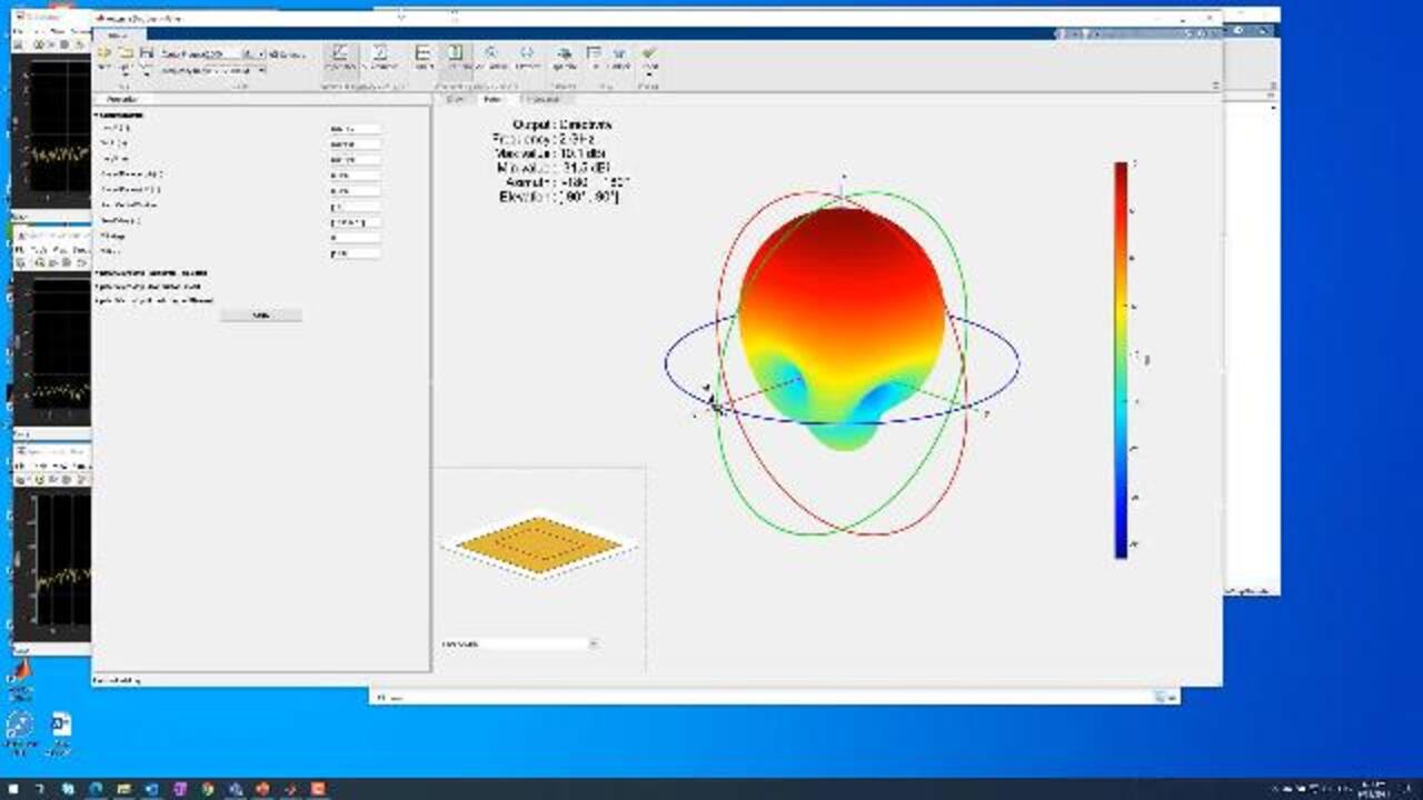
For example, let's look at the microstrip. And say we choose this particular element. The next thing that we see, what kind of backing structure-- here we already have a backing structure. This is a rectangular backing structure. And then, we specify what is the operating frequency-- two gigahertz. So then, you click accept. Now you get the power strip antenna. And you can specify or revise its length with height, things like that. And then, you can go ahead to perform analysis. For example, look at the impedance, you look at the radiation patterns of this particular power-- patched microstrip element.

So this is the patched microstrip of this particular patch micro with these physical parameters. You can do many, many other things, for example, look at the impedance of this particular patch microstrip, and how it changes at different frequency point. So again-- by the way, the antenna toolbox uses mass of the moment EM Solver to obtain a different-- to perform desired analysis, such as look at the impedance, look at the S parameters, look at three dimensional patterns.

So one particular use for features of this app is, once you design the antenna, then you can export it. You can export it back to the workspace, or export it as a script. So next time, when you want to design the element, you don't have to go through this interactive process again. You simply run the script. So if we export the workspace antenna, you will get something, for example, you'll get an object in the workspace. And you can also export it as a script. And by running the script, you can get all kinds of things, for example, antennas, object, you get the impedance characteristics, and also the patterns. So whatever you have done interactively, by running the script you can get it as well.

So once we designed the element, there's a number of ways to design antennas from the individual element. So one way of doing that is to import the antenna element radiation pattern into the sensor array analyze, which we looked at earlier. For example, in the previous example, when we look at the six element uniform linear array, the radiation pattern is from the custom antenna with this mechanoid pattern specified by this MATLAB variable PAT.

So when we design antenna element, we simply running it, analyze it, obtain the individual element's radiation pattern, and if it expressed, use the MATLAB variable. In this particular case, it's a PAT. And then, you just load into the Sensor Array Analyzer. Then we can use this custom antenna element to build an array of antennas and perform array analysis as we did in the previous example. And it can also use another app, called Antenna Array Designer to perform-- to construct an array of antennas.

So the difference between the Sensor Array Analyzer and Antenna Array Designer, is that when you use the Antenna Array Designer, you are using this EM solver-- MOM-- Mass of the MOMENT EM solver to analyze-- to calculate the radiation pattern of the array. So in that case, the coupling effect, energy effect, and all kind of additional effects will be taken into account. However, because of the EM solver-- because of the complexity of the EM solver, the analysis or calculation will take much, much longer.

So we will not go into this Antenna Array Designer today. But feel free to explore it once you-- if you have access to this tool. So another thing that I wanted to mention is, in the latest release, 2021A, antenna toolbox introduced another computational technique called fast multipole method. So this is very, very powerful and useful technique introduced in this new release.

So the FMM provides an effective way of modeling and analyzing antennas and array on large platform. The key advantage of FMM is that it reduce the memory requirements and increases analysis speed. So if you are running into this memory or speed issues, make sure you are upgraded to the latest version so you can take advantage of this FMM technique.

And also, there are lots of additional extensions to this antenna design workflow, such as optimizing antenna performance, importing antenna data, modeling custom antenna structures, and the modeling the effect of antennas on larger platforms. So there's a lot of examples in the document. So feel free to look into them and study further.

So now, let's move on to the third topic today, RF front end design and architectural exploration. As we have seen in the first example, shown at the very, very beginning of the seminar, including RF modeling helps accurately simulate and predict the system performance. Also, signal processing algorithms can only be made effective and robust when various RF impairments are taken into account.

So one critical issue encountered for simulating RF system is the simulation time step. So RF transit simulation requires time steps to be commensurate with the RF carry frequency. On the other extreme, time steps for baseband physical layer simulation are determined by the broad bandwidth of the generated waveform, which is typically way bigger than that for RF simulation. The small time step poses many serious and sometimes insurmountable issues, which most of us should be able to appreciate.

To overcome the difficulties, some compromise or trade-off is necessary. To enable fast and accurate RF system simulation, RF block set provides circuit envelope. You can see, circuit envelope as a generalization of equivalent baseband, where you can efficiently simulate a signal with a sparse spectral occupation using multiple frequencies. RF Blockset is a unique system level simulator, as it allows you to choose which simulation technique to use, and it operates on behavior models rather than transistor level implementation.

RF design and the modeling is complex. So where to start? Again, MATLAB Simulink RF modeling tool has an app for you, called RF Budget Analyzer app. The bullets in the slides summarize its capabilities. Let's take a look at the app. So we still go to the signal processing and the communications section, and look for the RF Budget Analyzer. So again, this is the same thing as the other app. On the very top is your toolstrip, so you can start off with a totally new RF system, or you can open from the existing ones. Or you can build it from scratch yourself.

For example, you can say, OK, I'm working on some system, which is operating at 2.1 gigahertz. The incoming signal's power is at the minus 30 DBM, signal bandwidth 100 megahertz. So for example, the next the section is basically the RF devices or components. For example, you can start with a SMS parameter, which basically is nothing but some from end bandpass-- could be some bandpass filter. And followed by, say, a low noise amplifier. So for each of the component, you can change the name. For example, a low noise amplifier. You can specify the gains, say 12 dB, noise figure, 2.3, things like that.

And by this approach, you basically build up your RF system component chain. So for example, I already have something I already worked on before. So I can open it up. So we say, open. Save current, say no. RF component, So this is a five component RF chain.

And notice that the RF Budget Analyzer actually does not do any numerical simulation. Instead, it uses some formulas to calculate say, gains or power levers at each stage of the RF chain All this noise figure, IP3 values to noise ratio is computed using some formulas. So this is give you a very, very quick way to evaluate your RF chain, to determine the signal to noise ratios at a different stage of the chain.

So once you're happy with the system, you can either export it into a workspace, or export it to RF block set, so you can simulate with your other system Simulink model. For example, you can export it into the RF block set. You can insert it into your baseband communication system model. Either put it on, for example, on the receiver side, things like that.

So this is a very quick ways to perform our budget analysis using the RF Budget Analyzer. So basically, you can do all kind of analysis. For example, this amplifier file, showing in 3D-- three dimensional scenario, for example. Shows the power levels across your band of interest for different stage. So all of this analysis tools are built into the app.

So you can also export it, as I mentioned, into an RF block set, and then just insert this whole part. So this is a Simulink interface. This is another Simulink interface. So you can place-- insert into your physical layout, or baseband Simulink model. So one question, at this point you might want to ask is, may I do all of this in MATLAB? Because say, my model is written in MATLAB, and I'm not very, very familiar with Simulink. Can I do all this RF budget analysis in MATLAB?

So the answer is yes. With the release 2021A, the tool adds a system object, called RF system. So here are the examples how you can build a Budget Analyzer object, and use this RF system to run it. To specify input, simply say, RFS of IN. IN is your input-- the time domain signal for the RF system. Then you get an output. So all this Simulink numerical calculation or simulation is basically-- this is running behind things. So you don't have to open Simulink at all.

So this is an example in the document. You can take a look at it, and to provide a lot of convenience, especially for those who are not familiar with Simulink, and who don't want to go into Simulink. So this is a great tool. Again, there's many, many examples in the document. So if you want to learn more about RF modeling, the help documents for RF toolbox and RF Blockset are always a good place to start. More examples there address many other aspects of RF modeling that we did not have time to discuss today.

So to summarize what we talked about today, I do want to mention that due to the time limitation, we did not have the opportunity to go as deep or in as much detail as you would like to. My hope is that you could carry this tool tips away with you when you work on any projects that are related to antenna, phased array, or RF systems.

You may open the slide deck from today's presentation and check out some of the examples we talked about today. If you ever need any help from us, please do not hesitate to let us know. We are here to provide all necessary assistance for you to succeed. All right. Finally, is a reminder, we have our last session of the webinar series on July the 1st, developing with and deploying to software defined radio--