Wireless Scenario and System Design | Developing Next-Generation Wireless Communications for Aerospace and Defense

Hello, everyone. And thank you for joining our first session of the wireless series for aerospace and defense My name is Mo Alsaleh. I'm a senior application engineer at MathWorks. And my area of expertise is mainly wireless communication. The first session will be talking about wireless scenario and system design.

Here is our agenda for the first session. First, we will define the term scenario. Then we'll show you how to model it in different ways in MATLAB. We will explore different propagation models and analyze coverage with and without terrain consideration.

Then we'll move to urban environment and use ray-tracing techniques. And through this journey, we will be showing you what we have added in the latest MATLAB releases. Finally, will switch from terrestrial communication to space communication with our new satellite communications toolbox before concluding the session.

Let's start by looking at the big picture. So a wireless system will have different parts. We have digital baseband waveforms, then processing, then go into to analog IFs and the RF domain, and finally, transmit over antennas. Then a channel, and back through antennas, analog domain, and baseband processing

And you see that we have different tool boxes to support you at each stage. Whatever your rule, is, you can use this slide as a reference to find which tools you might need for your future tasks.

Today, I'm focusing on the link analysis-- basically, everything that goes outside your transmitter. So in session two, we will be talking about the end-to-end systems and focus on the digital baseband portion of it. In part three, we'll be talking about the RF and antenna pieces.

And in the final session, we'll be talking about the application and hardware implementation, things like software-defined radio So basically, level modeling covers everything outside the transmitter and receiver, things like RF propagation, link budget calculation, and overall coverage.

Let's define scenario modeling and see why it's so important. So what is a scenario? This Department of Defense definition says that it's a conceptual description of how major system or players interact with each other for a given environmental conditions.

And the wireless domain systems can be transmitters, or receivers, or even obstacles, where relations can be linked budget equations, propagation models, and conditions can be weather conditions, or environment nature.

So why it's so important to do scenario-level modeling, first, to check the feasibility of the design, to check if it's doable or not. So if you're in R&D or a design engineer and trying to get the proof of concept before applying for funding or filing for a patent, for example, you need to do so.

Once you have your basic design, you will need to decide on the minimum power, antenna size, the number of elements. All of that can be done with the budget analysis, as those parameters usually utility cost you the most.

Then move on and decide on the quantity and quality of the rest of the components from the simulation results. That's before going into field testing and spend more time and money on the field tests.

You finally run the dynamic scenario and visualize it to make sure you did not miss any crucial design requirement. Or also, it can sometimes trigger new ideas.

So let's see how to model RF propagation over terrain in MATLAB using the antenna toolbox. So the antenna toolbox has many capabilities beyond designing and analyzing antennas. So you can visualize antenna coverage and calculate a different system performance metrics, like signal-to-noise ratio and signal-to-interference-and-noise ratio.

You can analyze coverage and visualize it on different kind of two-dimensional and three-dimensional maps. And you can also exploit the different propagation models in the literature, like Longley-Rice model or TIREM model. And finally, you can also use beam-steering to enhance coverage or track users, as well as you will see in the next example.

Let's got to documentation. I want to show you how you can reach our example. So if you go to MathWorks.com, this is the main page. If I click on Support, and then Documentation or Examples, both of them will take me there. I could see the list of the toolboxes they have alphabetically.

You can see the list of toolboxes I have arranged alphabetically. So if I click on the antenna toolbox, it will take me to that toolbox. And I have everything listed here. If I click on the Examples tab, I'll be able to see the different categories of shaping examples that we have in that toolbox, and we'll be looking at the RF propagation.

And we'll be starting with this example called RF Propagation and Visualization. So let's click on that. And I want to scroll down and just show you the story of this example.

So in this example, we'll be importing a realistic map for Natick, Massachusetts area, where we have our main campus. We'll be setting a transmitter on this GL map here and red. We'll be setting up a receiver also a few miles away, and study and analyze the communication link between them after setting the antennas, transmitter antennas, the receiver antenna. And later on, we'll be plotting the coverage map. And we'll be adding an interference source, and consider the terrain to make it a more realistic scenario.

So how do you open it in MATLAB? If I scroll up, in the top right corner here, View MATLAB Command, if I click on that, there will be this command. And I'll take it now to MATLAB. And in the Command window, I'll paste .

So just like any of our shaping examples, every shaping examples starts by a brief description of the goal of that example. So this example shows how to compute and visualize outdoor wireless coverage between a transmitter and the receiver. So let's run it section by section and see how to set up a basic wireless setup.

So the first step would be to set up a transmitter. And you can see we're using the system object called txsite. All what you have to give it is the latitude, longitude, and give your site a name. So let's run that.

Now MATLAB will be using a tool called Site Viewer, which is embedded in the antenna toolbox, that opens that map and locate the transmitter here in read on the longitude and latitude that the user gave. So this is the transmitter here in red. This is our main headquarter, the one I'm talking to you right now from. And we'll be setting the transmitter on this one.

The next step would be setting a receiver. And we can do it the same way with our rxsite system object with the latitude and longitude. And with the receiver, now we have to provide things like receiver sensitivity. We can determine our parameters like the antenna height, the type of antenna-- so isotropic.

And we use the same thing for the transmitter isotropic, antenna for the transmitter. 2 gigahertz of frequency, so you can tell we're trying to simulate a low-frequency system like LTE or 5G sub-6. Transmit power, ten watts.

So let's run this. And now the Site Viewer will be updating this map with the receiver here in blue. Next, MATLAB will do all the calculations for us. So it will calculate the distance between the transmitter and the receiver based on both locations. And it will calculate also the angle between the transmitter and receiver, just in case we're using any beamforming techniques.

And as we have the gains for the antenna transmitter and the antenna at the receiver, and we know the distance and the transmit power, we can calculate the path loss. And you can see that MATLAB calculated the received power at the receiver. And since we provided the sensitivity of the receiver, calculated also the margin. And we can see that here. It is in green.

Next we'll-- using the link that includes the transmitter and receiver, will plot the link quality between the transmitter and the receiver here on Site Viewer. And it's color-coded. Green means we have-- the transmitter has delivered enough power above the sensitivity of the receiver that we picked. If the transmitter were not able-- was not able to deliver enough power above the sensitivity, this link would be indirect.

Of course, you can change the format of the map. So you can pick a lighter one with street names, you can zoom in and out. And you can do a lot of stuff with the site view.

Next, we'll be plotting the coverage map for this cell. And we'll use the function called coverage. We'll have to determine the range of power that we want to plot so simulation does not take forever.

And now MATLAB will be plotting the coverage of that transmitter that we put on the same map with this power scale. You can tell from this plot that we have two consideration in mind. So for our first, that we're using an isotropic antenna at the transmitter, just like what we configured. And this results of this kind of ideal spherical coverage. The second consideration that we have not considered any terrain so far.

Next to make it more realistic, if you remember, we used almost 2 gigahertz at the transmitter frequency. Now, we'll be using this frequency and setting up another transmitter to simulate an interference source. So Site Viewer again will set up another transmitter here in red.

And we will be recalculating now the signal-to-noise and interference ratio-- not only signal-to-noise, ratio like the first step. And we'll be also now considering the terrain in that spawn cell. And the default propagation model, that's considered there as the Longley-Rice Model.

So MATLAB now will be updating the coverage map with the interference source, with considering Longley-Rice source that include obstruction and diffraction. This was our first example for today. Don't forget to close the Site Viewer once you leave it and clear all other values.

And here are more coverage analysis examples from the toolbox, just for your reference. And now let's move on to different method of coverage analysis, the ray-tracing techniques and different type of environment-- urban environment.

So in the previous example, we used low frequency, we used omnidirectional antennas, and open space area of interest. That is usually the case for LTE or 5G sub-6. Now for millimeter wave, as the frequency of operation is higher and around 28 gigahertz, modeling will be different in many aspects.

So it will demand more precise RF propagation modeling. As the frequency is higher, the path loss will be also higher. And so millimeter wave suits shorter distance links. And typical environment for these users will be urban environments.

When you're working with urban or suburban scenarios, you need building data. One open source for building data is OpenStreetMap, which is free, open, and crowdsourced database. Next I'll show you how to import a map from OpenStreetMap and use ray-tracing methods that we added in our 19B to study the coverage in the Canary Wharf district in London. This 19B ray-tracing capability model reflections only and uses the perfect image method.

So if I open a new tab here and go OpenStreetMap.org, in the search window, I'll put Canary Wharf and hit Go. Then I can click on the Export tools, and I can see the latitude and longitude. I can click on Manually Select a Different Area and try to concentrate my area of coverage on Canary Wharf. And once I'm done, I can Export. And since I already did that, I'll just close this. And you can save this on a local directory and open it with MATLAB.

So the second example today, I'll show you how to find it. So I'll click on RF Propagation and Visualization again. Examples, and I'll scroll down. And it's called Urban Link and Coverage Analysis Using Ray-Tracing. So we'll open it the same way.

Go to MATLAB and open it. So this example shows how to use ray-tracing to analyze communication links and coverage areas in urban environments.

So the first step would be to set up a transmitter, just like what we did in the first example with the latitude, longitude, antenna height, and deciding how much power we want to transmit. And I noticed that the frequency range has changed now from low frequency to the millimeter wave. Site Viewer already open that map that we opened and saved from OpenStreetMap and set up the transmitter for us in red again.

Next, I will view the coverage map for the line of sights only, on that map. And the first one where we have line of sight only the. And for that, we will be using the coverage function. Will determine the resolution, the signal strength, just like what we did in the first example.

And MATLAB will be updating the coverage map on Site Viewer now. While MATLAB's doing that, we're going to set up a receiver site the same way-- latitude, longitude, antenna height of 1 meter, to simulate a user going around that cell. And now we can see the coverage for that cell in the Canary Wharf considering only line of sight in this power range.

Next we'll define a receiver close to that transmitter by providing the longitude and latitude. Again, just like what we did in the previous example. And notice that now MATLAB loads the direct link between the transmitter-receiver and we do not have line of sight between them. And of course, we did that on purpose so we can use the ray-tracing technique and analyze the link with one or many reflections.

Next step will be plotting the propagation path for one reflection. This is the shortest path after the line of sight. And you can tell from the color that the received power is around minus 80 dBm. And we considered a perfect reflection material for this building that reflected the signal.

Next we will consider a more realistic scenario, and we'll pick a material for this building, which is concrete in this case, and as a result, will be losing some dB as a reflection loss. We'll also include some weather losses. And MATLAB can help you decide on the different losses that's caused by rain, gas, and you can even determine the rate of rain, or snow, or so on.

And as a result, our received power is now going down. And if you notice, it was minus 78 before the weather losses. So we lost almost 1.5 dB for the weather here. And from minus 70 to minus 79, we lost about 9 dB for the material loss.

Next we plot the coverage map for a single reflection path for the whole cell rather than just for the receiver. And again, Site Viewer will update the coverage map on that cell for us.

So notice that we did not have any coverage between these two buildings because we did not have a line of sight. The same thing was behind those obstacles. We did not have any coverage, but now we have at least minus 80 dBm of received signal because now we're considering the reflection from other buildings, and we're considering one ray of reflection so far.

Next we will consider two reflection rather than one and we'll see how the coverage map will be different. And you can see that we have two different paths now. One of them is a little stronger than the other one because of many reasons-- mostly because it goes through a longer path.

And now those will be added of course, constructively or destructively based on the phase at the receiver. And in the next step, we'll be plotting the new coverage map for the whole cell using two reflections rather than just only one.

And as you can see, once we have two reflections, now we have a better signal in those non-line of sight spots. You have darker blue in those spots that we did not have any line of sight. And we have lighter blue, which means more signal in those spots that used to have like darker blue with single reflection only. That means they receive now more power .

Next we'll update it with four reflections. And with that, we expect more power, of course, at each spot. And you can see that the whole coverage area of our cell is almost covered with a certain level of signal.

And this last step, now we want to enhance our coverage, just like a millimeter wave and 5G systems. And now we want to use a directive antenna, which is a phased array antenna that's using 8 by 8 uniform rectangular array of elements rather than this omnidirectional antenna. And we will be updating the coverage for the receiver first.

And with this directive antenna that we built with the first array system toolbox, now we'll plot the shortest path between the transmitter and receiver and see how millimeter wave will help updating the coverage for that receiver in that spot.

So as you can see, this receiver that used to have minus 90 or minus 80 dBm with a single reflection, minus 80 to minus 70 with two reflections, and a little better than that with four reflections, now with a single reflection only with this directive antenna, now we jump to minus 50. So we gained almost 20 dB. And you can tell that this 20 dB is most probably the gain of the phased array.

So this example, again, showed us how to use ray-tracing techniques to study the coverage for a single receiver or for the whole cell coverage area using an omnidirectional and a phased array antenna on the millimeter wave frequency range.

OK. We always recommend that our customers move to the latest release of MATLAB to make use of all new features. So let's see what we added in the latest releases.

As I said, the perfect image method was added in our 19B release and 21A release, we have added the Shooting-Bouncing-Ray, SBR, method, which is much faster and supports up to 10 reflections. If you need to learn more about both methods, you don't need to leave our documentation to do so. The reference page I included here at the bottom has all what you need. So let's click on it quickly and see what this page in our documentation gives.

It shows you how to model all kinds of atmospheric losses using rain, free space, gas, fog, frequency range of each the references that we considered for each model. Also for the terrain models, we talked about Longley-Rice, we used it. If you want to use TIREM, here is the difference between both in terms of frequency range, in terms of limitations, and so on.

And here is the two ray-tracing techniques that we have in MATLAB, the perfect image and the shooting and bouncing rays, the difference between them, the frequency of each, and even if you need to go through the algorithms of each and try to understand. Again, this page is listed here as a reference for our users.

We have been talking about terrestrial communication systems like LTE and 5G. Now we will switch to space communications.

So our first example is from our sensor fusion and tracking toolbox, which is 2020B example, where we build a space debris tracking scenario. In this example, we have got four radars that are based on the ground looking up into space. Those white dots here around represent space debris that we have generated orbits for.

And what you will see is as the debris passes through the radar coverage and detections are generated, those detections will be converted into tracks through the tracker. And as those tracks exit the radar coverage, the uncertainty of those measurements will start to grow until we get another measurement, and so on. Hopefully the detection will be generated when it passes through the next radar.

So let's run this again and explain the whole scenario. So again, as the debris leaves this radar coverage, this uncertainty keeps growing up because now the tracker does not receive any detection for this debris. And this uncertainty ellipse keeps growing in size until this kind of debris goes into the next coverage area, and now we get detections again.

Now we have four different coverage areas, and as you can see, as those debris goes through the radar coverage area, we start getting detections from the radars for them. And we feed that to the trackers. The tracker can create those different tracks that has [? T ?] and two-digit numbers.

And as those debris leave this coverage area of radar, we won't be able to receive detections anymore. And that's why the uncertainty will keep growing until we fall into other radar coverage and start receiving detections again.

What's nice about this is you can generate scenarios that would be hard to otherwise recreate yourself. And this allows you, in this example, to set up the radars, set up the trajectories of the objects that are in the field of view, and also test the tracker to see how they output.

That was our first example in space communication. The second example is from the new satellite communication toolbox, which we added in our 21A release. This new toolbox enables us you to simulate, analyze, and test satellite communication systems.

It comes with many features that we cannot cover today. But one of those features is satellite scenario generation and visualization. The toolbox provides the ability to read TLE files and generate an orbit from that file. TLE files can describe the orbit of one or many satellites, and they are commonly used across the entire satcom industry.

You can use these TLE files with SGP4 or SDP4 propagators, or you can use it with the Keplerian two-body model, which is less accurate than the SGP4 and the SDP4, but still very useful for an engineer just starting out with the orbital mechanics.

The toolbox enables you to visualize in either 2D or 3D. You can generate different fields of view, which can either be constrained or unconstrained by a ground station, minimum elevation angle, and satellite maximum steering angle. And you can also visualize ground tracks to obtain a quick picture of the coverage area of satellites over multiple orbits around the Earth.

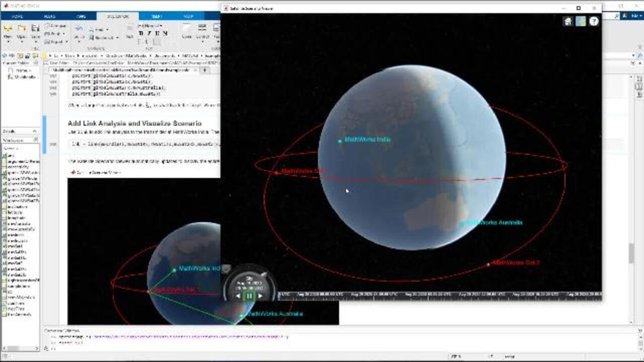
The last wireless scenario which we will build today would be a satellite communications scenario. And in this example, we will set up a multihub satellite communication link between two ground stations. The first ground station is located at MathWorks India and the second station is located at MathWorks Australia.

The link is routed via two satellites, MathWorks Satellite 1 and MathWorks Satellite 2. Each satellite acts as regenerative repeaters, which receives an incoming signal and then demodulates, remodulates, amplifies, and finally retransmits the received signal. In the last step, we will calculate the times over the course of a day during which MathWorks India can send data to MathWorks Australia .

So let's move to our Documentation page again. So if I click on Documentation Home, and I can see all the toolboxes again. I'll scroll down Satellite Communication Toolbox Examples. And here is our second example from the satellite world for today.

all our shaping examples starts with a brief description. So this example demonstrates how to set up a multihub satellite communication link between two ground stations. So and the first step would be creating a satellite scenario. And a satellite scenario is nothing but the container where you give MATLAB the start time of stimulation, the stop time, and the sample time, which is how often you want MATLAB to generate the output for you.

Then we launched the Satellite Scenario Viewer. And the Satellite Scenario Viewer is just like and the Antenna Site Viewer that we saw on the antenna toolbox. So MATLAB will open that and we will be able to locate the different components of the satellite communication links like the satellites, the ground station, the orbits, and so on.

So this is the Satellite Scenario Viewer. You have too many options as well for visualizing 2D or 3D, different kinds of maps you can change between them. Once we have the Satellite scenario Viewer open, we can start adding satellites. So we'll be adding the first satellite with all the parameters that we got from a TLE file, for example.

And you saw that we picked an eccentricity of zero, for example, then that tells us that this orbit will be circular. So that's one way visualizing this the scenario help you make sure that you pick the right parameters, help you understand the scenario, and make sure that you did not miss any points.

We add the second satellite the same way. And the Satellite Scenario Viewer will be updating that right away. Next, we add the gimbals to those satellites. And gimbals is nothing but that mechanical part that holds and steers the antennas.

Once we have gimbals, we will be adding receivers and the transmitters to these gimbals. For the receiver, we'll have to pick the gain-to-noise ratio, the required Eb to end node ratio for the performance. And we'll be using a Gaussian antenna, the default antenna that comes with the satellite communication toolbox. The Gaussian antennas is a multilink-- a parabolic dish antenna which is the most commonly used antenna in satellite communication.

You can pick a higher diameter here, which gives you more gain and narrower beam if you want. And you can replace these two lines of codes with any single line of code from the antenna toolbox box or the phased array system toolbox if you have access to them and use a different antenna or antenna beam techniques if you want.

Next we'll be adding the transmitter, and picking frequency of operation, and how much power we want to transmit at each satellite, and adding antennas to those transmitters, just like what we added to the receivers. And now once we're done, or almost done, with our satellites, now it's time to add ground stations.

So the first one is MathWorks India. And just like what we did in the first antenna toolbox example, we just provide longitude, latitude, and the name of the site. So we add MathWorks India. And here we go, we see it on the map. Then MathWorks Australia. And the Scenario Viewer updated right away.

Next we add gimbals to those ground stations, just like we set them up on the satellites. And the same way we add transmitters to those ground station, mainly MathWorks India because it's a one-way communication. And we had an antenna for the transmitter at MathWorks India.

Then we had the receiver for MathWorks Australia, which receives only. And we add an antenna for the receiver at MathWorks Australia. Then to save you the effort and the time of writing a tracking algorithm for those antennas, we provide a function called pointat where you tell each gimbal where to point exactly.

And in this scenario, we need six gimbals. I'll show you quickly on the Satellite Scenario Viewer why we need six of them in this case. So remember, we said it's a one-way communication. So MathWorks India is trying to transmit to MathWorks Satellite 1, Satellite 1 to Satellite 2, Satellite 2 receiving and then transmitting to MathWorks Australia.

So we need the first gimbal at MathWorks India to transmit or point at Satellite 1. MathWorks Satellite 1 will be using two gimbals, one at the receiver to point at MathWorks India and receive from it. And the other one at the transmitter that points to MathWorks Satellite 2 and transmit to it. And so on, we need 1, 2, 3, 4, 5, and the last one is at MathWorks Australia to point at MathWorks Satellite 2 and receive from it.

Then we add the link and we put those four major components that we have on the Satellite Viewer, the two ground stations and the two satellites. As you see, it's updated.

And next we'll determine the time when the link is closed and visualize this link closer. So for the link to be closed, first, you need a line of sight in this scenario between any transmitter and receiver. And second, you need to deliver enough power at the receiver site so the receiver can decode your signal.

And you see, now MATLAB generated this table for each source-- MathWorks India in this case, target MathWorks Australia in this case. When we had those links closed at what time started, what time ended, and for how long in seconds. So if you multiply these duration in seconds by your data rate bit by second you can tell during that day how much data you could transmit between MathWorks India to MathWorks Australia.

In the next step, we'll play the scenario and we'll show you how MATLAB did all of that. You can visualize the scenario and see what parameters affected that. So let me zoom in here-- or zoom out.

As you can see, as long as you have line of sight between the four components and you deliver enough power for the receivers, we will have a green link. That means the link between MathWorks India and MathWorks Australia is running and up. Once we lose line of sight, now the whole link is broken. And you can tackle that as a communication engineer by adding more satellites with more orbits or trying to transmit more power while this link is up and running.

You can also modify your required Eb to end node. Increase it and see how the performance change or decrease it and see what other parameters will change accordingly.

That was our last shaping example for today. Let's see if we can summarize it and see what we have looked at so far.

So to summarize, we have seen how to model different wireless scenarios with different types of antennas and their activity. We visualized coverage on different kind of maps with and without considering terrain. We set up different satellite links, measured the closure time, generated tables and charts for those durations, just like what we saw in the last example.

We also visualized all what we have mentioned so far in those scenarios. And finally, we calculated the different link performance in terms of signal-to-noise ratio, signal-to-noise-and-interference ratio, like in the first example, bit error rate, and you can translate all that to throughput.

This is where we started this series. Today, we covered scenario modeling. The related toolboxes are highlighted here for your reference.

The next session, [? Hohmann ?] will go through end-to-end systems. In the third session, [? Neal ?] will go through RF and antennas. And Rob will be closing this series with hardware implementation. We hope to see you next time. Thank you for watching.