Enabling RF Circuit Envelope Simulation in MATLAB

Welcome to this presentation, where I will be discussing how you can increase the fidelity of your wireless waveform physical layer simulations by including RF impairments that are modeled by a RF circuit envelope simulation. This level of RF impairment modeling is not included in MathWorks Communications Toolbox nor the standards compliant tools, such as 5G Toolbox. This additional level of RF impairment modeling facilitates better designs of baseband receiver demodulation algorithms along with adaptive transmitter linearization.

I will be covering the three elements that comprise the workflow to perform RF circuit envelope simulation in MATLAB. First, I will discuss how you can use MATLAB to generate wireless waveforms, whether they are standards compliant waveforms-- such as those that are compliant to the 5G, wireless LAN, or LTE specifications-- customized waveforms that can be generated using Communications Toolbox, or waveforms used in radar applications, such as those used in pulse, FMCW, or PMCW radar.

We will then discuss how you can use a MATLAB application called the RF Budget Analyzer, which is part of MathWorks RF Toolbox product, to develop a RF front end, whether it be in a transmitter or receiver. Then the cascaded RF network will be exported to MATLAB, where it will be subsequently turned into a System object that supports RF circuit envelope simulation in MATLAB scripts.

Then I will show you how you can modify your MATLAB Test Bench script to increase the fidelity of your physical layer model by inclusion of the RF circuit envelope object generated from the RF Budget Analyzer. As you can see on the accompanying figure, this workflow can be used to model sophisticated RF front ends, such as those that you would find in receivers with Automatic Gain Control or transmitters with power amplifier linearization.

Before we get into the technical part of the presentation, I would like to spend a few minutes discussing how MathWorks tools can be used in behavioral modeling of end-to-end wireless communications systems. Over the past number of years, MathWorks has made continual investment in the wireless communications design space. MathWorks offers products that span each aspect of wireless communication system design, including tools for wireless standards, physical layer modeling, as well as validation and verification. With the 5G, Wireless LAN, LTE, or Communications Toolbox, you can prototype and develop standards compliant waveforms that you can subsequently integrate into physical layer simulations.

With application-specific add-ons, the standards compliant waveforms can be virtually tested in the presence of RF impairments, adaptive algorithms such as those used in beamforming or power amplifier linearization, along with the behavior and free space realized by channel modeling and RF propagation techniques. Also, full-wave 3D electromagnetic analysis of antenna elements and arrays can be integrated into the system model so as to more fully evaluate adaptive hybrid beamforming algorithms, allowing you to validate the beamforming strategy before transitioning to a hardware implementation.

We are going to be focusing the presentation today on how we can integrate common standards compliant waveforms along with detailed RF front end models to evaluate common architecture, such as those used in power amplifier linearization, along with hybrid beamforming. Digital communications engineers are accustomed to using MATLAB for waveform generation prototyping along with development of signal recovery algorithms, such as carrier and timing recovery.

MathWorks standards toolboxes support RF impairments such as odd order, nonlinearities, and phase noise. However, they don't support frequency-dependent behavior or even order nonlinearities. RF system architects typically work in a drag and drop, block diagram environment and commonly describe system behavior in terms of frequency-dependent descriptions, including small signal linear behavior, noise, and nonlinear performance. Uniting these two workflows into a single, unified workflow would facilitate better communication between the digital communications engineer and the RF system engineer.

On the accompanying slide, you can see a typical example of how a digital communications engineer would use MATLAB to prototype a wireless waveform along with a receiver for decoding. On the left-hand side of the slide, you can see how a 5G new radio waveform can be generated, where containers are instantiated to include information such as channel bandwidth, subcarrier spacing, number of resource bits, as well as information about synchronization signal burst. On the right-hand side of the slide, you can see how MATLAB can be used to prototype a baseband receiver or channel estimation, resource extraction, as well as calculation of peak, and RMS error vector magnitude is performed.

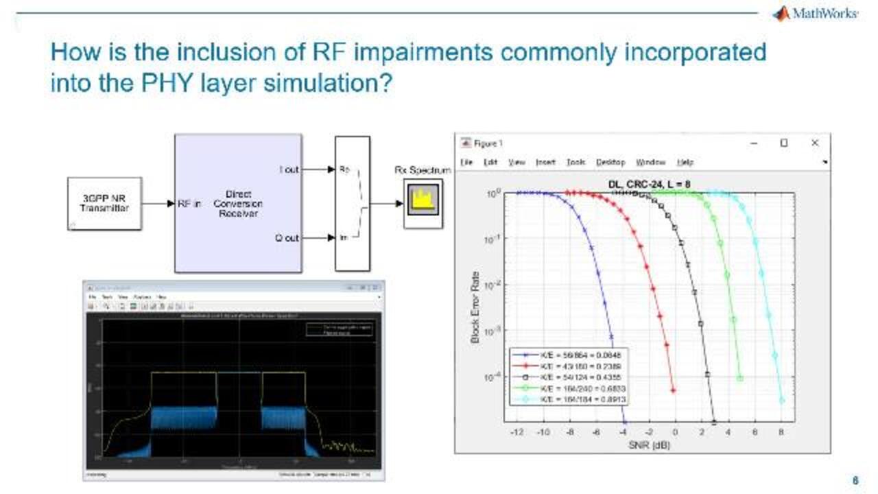
Conversely, RF system engineers use a drag and drop environment to model the RF front end. A typical example is shown on the accompanying slide, where RF system engineers would do architectural exploration of a RF front end being driven by a standards compliant 3GPP new radio waveform. The 3GPP new radio waveform would typically be realized in the frequency domain and then pass through the RF front end of either a transmitter or receiver, and the output waveform would be captured on a spectrum analyzer.

Based on the signal to noise ratio and any of the bit error rate, packet error rate, lock error rate, or chip error rate, the throughput of the RF front end can be evaluated. Based upon a desired error rate, specifications for both the overall RF front end along with respective components within the RF front end can be determined. For instance, the gain, noise figure, and inner modulation product performance of a low-noise amplifier can be determined using this type of analysis.

As we saw in the previous two slides, base band digital comms engineers are accustomed to working in a programming environment, while RF engineers are accustomed to working in a drag and drop, block diagram environment. What we will now do is go through a workflow example where you can use MATLAB to do waveform generation, either by a scripting or through the Wireless Waveform Generation application.

Once the waveforms are generated, we will then use the RF Budget Analyzer that is part of the RF Toolbox to generate an RF cascade that permits you to model RF impairments such as frequency-dependent linear behavior, noise, along with non-linear behavior. Then we will use a new feature within our toolbox called the RF System object to perform circuit envelope simulation of RF systems excited by a standards compliant waveform generated by either the Wireless Waveform Generator application or standards compliant toolboxes such as the 5G, Wireless LAN, or LTE Toolbox.

To demonstrate this workflow, let's go through an example where we will use the 5G Toolbox to generate a 5G compliant waveform, specifically a downlink waveform operating at millimeter wave frequencies, and add RF impairments to this waveform via the RF System object. I will use MATLAB as the test bench where a script is used to generate the 5G new radio waveform.

The inclusion of an RF front end within the MATLAB Test Bench will be facilitated by the RF System object, which was created from the RF Budget Analyzer object exported from the RF Toolbox application. As you can see in the accompanying figure, I make use of a MATLAB Test Bench where a 5G waveform is realized. It is subsequently passed through the RF System object that makes use of MathWorks RF Blockset Circuit Envelope technology.

The impaired waveform is then passed back into the MATLAB script, where demodulation and decoding of the received waveform is then performed. Then MATLAB can be used to visualize both the spectral response along with a constellation plot. From each of these responses, we can characterize the behavior of both the overall physical layer model along with the RF front end.

Before we get into the example, I wanted just to go to the 5G Toolbox example page to show which script I'm going to be basing the work from. So the example script that I'm going to be following, or is going to be followed, is the 5G new radio downlink vector waveform generation example. This specific example goes and shows you how to go and specify a physical downlink waveform which contains both its shared channel as well as control channel information, along with synchronization signal burst demodulation reference signal information. So this example is fairly complete, and it gives you a good start point for going and constructing a downlink waveform via the 5G Toolbox in MATLAB.

Now let's go through our specific example. So I was supplied this example by a colleague of mine, and some of the nice things about this includes a parameter setup section, which helps you for going and doing specifications of your 5G waveform if you're working at FR1, which is below 6 gigahertz, or at FR2, which is at millimeter-wave. So the table that's included goes and provides information on-- for the given bandwidth of your 5G waveform, how many-- the number of resource bits, the subcarrier spacings that you're going to use for both FR 1 and FR 2. So a nice, handy resource that's available in this example.

In this next section, we're going to be setting up the container information for our 5G waveform. So we're going to specify parameters such as channel bandwidth-- which frequency range we're going to be working at-- the number of subframes, the subcarrier spacing, and the number of resource bits. Next, we're going to be going through the synchronization signal burst information. So we're going to be going and setting up parameters such as the SSB periodicity, the block pattern, as well as the frequency offset for the synchronization signal burst.

The next part, we're going to be going and specifying the bandwidth parts. So specific things that we're going to specify include the subcarrier spacing, the cyclical prefix, the number of resource bits, and if there is going to be any sort of resource bit offset. In the next section, we're going to specify the core set container as well as the physical downlink control channel container. You'll note in both instances that we keep these empty.

The next section, we're going to set up the physical downlink shared channel information or specify that. So we're going to specify parameters such as the bandwidth part, the random data source, the target code rate, the type of modulation that's going to be used, as well as the number of layers. In this next section, we're going to specify time domain aspects of our downlink shared channel, including the number of allocated symbols, the slots, the period, as well as the resource blocks.

In this next section, we can see if we're going to go and enable the rate match for the core set. And then, next, we're going to go and specify, for the shared channel container here, the demodulation reference signal information, including the number of antenna ports used, the mapping type, the configuration type, as well as any sort of power boost. Finally, we're going to be putting all of these containers together within the wave config top-level container, and then, via the Downlink Waveform Generator function, we're going to go and generate our 5G new radio waveform.

Once we have generated the waveform, we can go to the MATLAB Command Window and visualize the information for the 5G waveform from bandwidth part 1. So we can go and take a look at information such as the sampling rate, the number of FFTs, the cyclic prefix lengths, the symbol lengths, as well as the number of subcarriers, subcarrier spacing, symbols per slot, symbols per subframe, samples per subframe, symbols per subframe, as well as any sort of window overlap.

Now, to simultaneously improve the ACLR and also to set a step time that is commensurate with the required data rate needed for circuit envelope simulation, we're going to upsample the signal, or our 5G waveform. Specifically, we're going to upsample it by a factor of four. This results from the band-pass filter included in the simulation, which requires a time step commensurate with at least twice the bandwidth of the band-pass filter in the RF System object.

So let's go and upsample our waveform. Now, at this point, we can go and visualize the response of the 5G waveform in the spectral domain by viewing the response on the Spectrum Analyzer. We can see from the Spectrum Analyzer, we can see the improvement in the Adjacent Channel Leakage Ratio. We can get information from the Spectrum Analyzer including the channel power. Make particular note of the channel power level. We're going to be using this in the RF Budget Analyzer when we perform harmonic balance analysis.

These four sections are inserted into the MATLAB Test Bench to facilitate circuit envelope simulation in MATLAB. First, we call the RF Budget Analyzer object. In fact, this function call readily allows you-- or opens up the RF Budget Analyzer application that's part of RF Toolbox. Next, we can go and load in the previous RF Budget Analyzer object generated from the RF Budget Analyzer. And then these next two sections facilitate the RF System object simulation in MATLAB.

So first of all, we go and load a previously saved RF System object. We set the sample time to be commensurate with the oversampled step time that we've previously derived within this test bench. And then we can open up and edit the RF System object. We're going to be covering all of the workflow in more detail momentarily.

And then this section right here readily allows us to go and facilitate the additions of RF impairments onto our 5G waveform, specifically going and facilitating the circuit envelope simulation within this MATLAB Test Bench. At this point, we are able to execute the second step in the workflow, where the RF front end is developed for either a transmitter or receiver network.

So in the script, we're going to go and execute this function here, the RF Budget Analyzer for this particular object. So we're going to run this particular section right here. And what we'll see is the RF Budget Analyzer is going to open up with the results from a previous run. So before we get into the specifics here of the results, just want to give a bit of an overview here of the benefits here of the RF Budget Analyzer.

So RF systems engineers typically use a spreadsheet to evaluate RF front end. In essence, they go and calculate cascaded parameters such as gain, noise figure, IP3, signal to noise ratio. Each of these spreadsheets is distinct for a specific transmit lineup or receive lineup.

The RF Budget Analyzer goes beyond the spreadsheet, as is it is extensible, where you-- where, typically first in the use of a spreadsheet, you need to transcribe the results from the spreadsheet into a separate RF circuit design tool. From the RF Budget Analyzer, it's extensible by going and using this export capability that's part of the RF Budget Analyzer.

The RF Budget Analyzer supports both Friis and harmonic balance analysis. The harmonic balance analysis is very useful for the analysis of transmit front ends, to determine what level of compression the RF front end is working in for a given input power. Impedance mismatches are properly modeled in between the respective stages that comprise the RF cascade within the RF Budget Analyzer.

The RF Budget Analyzer also supports analysis at either a single frequency over a-- or over a band of frequencies. So you can either adjust the input frequency or these plots that are available. You can go and plot the response of cascaded parameters such as gain, noise figure, IP3, the S-parameters as well. And then we can also see below that, there's-- as part of this, there is a number of parameters that you can go and take a look at, in terms of the cascaded parameters, via Friis analysis or harmonic balance analysis.

So there is a number of elements that comprise the RF Budget Analyzer. So let's start more or less in the top-left here. The first thing that we-- you do when you go and set up an RF Budget object is, you go and select the input frequency, the signal bandwidth-- the signal bandwidth actually sets the step time for circuit envelope simulation-- and then the available input power. If you previously remember from the Spectrum Analyzer plot, we had the peak channel power of minus 4.4 dBm, and we're going to use that same input power here to determine if our RF front end is within-- is operating in compression.

Next, let's go move over to the right, here, where we have the respective elements here, the Modulator, the Amplifier, and the Filter that go and comprise our lineup here. You can see on the left-hand side here that we can go and specify behavior for each of the respective elements here.

So say, for instance, for the Modulator, we can go and specify conversion gain, Noise Figure, Output IP2, Output IP3, as well as the Local Oscillator Frequency, and then if it's performing up-conversion or down-conversion. For the Amplifier, we can go and specify parameters such as Available Power Gain, Noise Figure, and, again, Output IP2, IP3, as well as the Input and Output Impedance, to set the match or mismatch in between the respective stages.

And then the last element that we have is the Filter. So there is a subset, or there is a-- different filter types that are supported within the RF Budget Analyzer, being the Inverse Chevyshev, Chevyshev, and Butterworth Filter types. So in this case, we're going with a Bandpass Filter Response.

We're going and selecting a Filter Order of 5. It's going to have a Bandwidth here of approximately 200 and-- or 160 megahertz. The Passband Attenuation is going to have a ripple of 0.06, which goes and corresponds with a return loss level of 20 dB or equal ripple return loss level.

I'm going to spend a little bit of time describing how you can come up with a new lineup using the RF Budget Analyzer. So here on the left-hand side, there is this option here, New. And this, actually, New pull-down offers you canvases that you can start with.

So there is the Blank canvas, a Receiver template, or Transmitter template. So if we just drop a basic Receiver template in, we can see that it's a single-stage down-conversion where you have an RF Filter. In fact, the RF Filter, in this case, alludes to or is referencing a touchstone data file, an RF amplifier-- like we described before-- the Demodulator, a clean-up IF Filter, and then in IF Amplifier.

So we can go and add or remove elements from this cascade with ease. So here we have a number of elements that are available within the RF Budget Analyzer, the Nonlinear Elements, including the Amplifier, Modulator, Demodulator, and a Generic nonlinear block. Then we have Linear Elements, such as an S-parameter block, Filter, Transmission Lines, Series and Shunt RLC networks, Attenuaters, transmit and receive antennae-- and these actually work back with the Antenna Toolbox-- an LC Ladder as well as the Phase Shift.

So let's say, for instance, we just wanted to add in another filter and then another amplifier as well. So it's just as easy as going and adding these in, and you can go and construct a network of arbitrary length. We can also remove these elements easily as well. So we can just hit the Delete Element and Delete Element, and we're back to where we have the single-stage down-conversion.

You can see down below that there is the calculation here for the cascade here. So in the table, there's a listing of the output frequency after each stage of the cascade, the output power, gain-- transducer gain, noise figure, IP3, and signal to noise ratio. We can also go and visualize these results as a function of frequency here.

So we have these different plotting types that are available. So we have the 2-Dimensional Plot, the 3-Dimensional Plot, the S-parameters, the Plot Bandwidth you can select, and the number of points. So say, for instance, we just want to take a look at the cascaded noise figure. So we can select that, Noise Figure. And here we can see that we haven't specified any noise figure, but you can see at the output of each stage of the cascade, you can see the cascaded noise figure.

So the first one is after the-- is the noise figure after the RF filter, then the cascade of the RF filter and the RF amplifier, the cascade of the RF filter, RF amplifier, and demodulator, and then the final stage. We can go and visualize a 3D plot as, say, over a band of frequencies. So say, for instance, if we wanted to take a look at the transducer gain, we see we have a 3-dimensional plot where the x-axis here is the fre-- is the frequency of-- that the analysis is being done.

The z-axis is the gain level, and then the y-axis here goes and depicts which stage of the cascade that we're at. So after 1 is after the filter. 2 is after the cascade of the filter and the amplifier. After 3, the cascade of the filter amplifier and demodulator, again, all the way through to the output here, the green being the output after the IF amplifier.

And then we can also take a look at the S-parameter plot as well. So we can go and visualize the response both in the rectangular format, as we see in the center. We can take a look at the Smith chart on the left-hand side, and then on the right-hand side, we can see the Polar plot as well.

Within the RF Toolbox example set, there is an exa-- there is an excellent start point example for using the RF Budget Analyzer and the entire RF Budget Analyzer workflow. So this example is the first example within the RF Toolbox, which is called "Superheterodyne Receiver Using RF Budget Analyzer Application." So this example goes through an exhaustive development of a superheterodyne receiver.

So, you can see, there's the block diagram. Then there's the construction of the superheterodyne receiver using MATLAB scripting, specifying the parameters here for the lineup here in terms of the center frequency, bandwidth, the impedance, and it goes through all the way to the point of where you're going and using the RF Budget Analyzer application, going and taking a look at the response here as a function of frequency after each of the cascades, so gain, noise figure, and then where you can go and export this back to MATLAB or going and exporting to the RF Blockset Test Bench. An excellent example to get started in the use of the RF Budget Analyzer.

Now that we've gone over the operation or how the RF Budget Analyzer works, along with a product example, let's go and return to our specific case here. So in this scenario, I actually did the analysis for two different scenarios. So there's, first, the basic analysis facilitated by the Friis analysis, which is just doing cascaded calculations based upon linear assumptions here.

So here we can see the basic calculation here of the cascaded gain, output power, noise figure, output IP3, and signal to noise ratio. You'll note that I had specified a fairly high input power here, minus 4.4 dBm. And we can actually go and use the Harmonic Balance Analysis capability that's been recently added to the RF Budget Analyzer, and we can see that there's actually a bit of a difference here between the results from the harmonic balance output versus the Friis.

And we're actually-- because of the IP2 and IP3 values that have been specified, the lineup is actually running in compression. In fact, it's very close to operating at the 1 dB compression point, so we're-- so the network is in mild saturation. So we can actually see here, based upon the harmonic balance, what the actual output power is, in this case, about 14.75 dB. The gain is 1 dB lower than predicted by the Friis transducer gain. The noise figure is reduced down a little bit as well.

And then we can see the new values here for the output IP3. We can see that's a lot lower than what was predicted by the Friis equation, but we can see that there's actually a little bit of an improvement here in the signal to noise ratio, so analysis that's very good in assessing the performance of transmit front ends that's facilitated here with the RF budget analyzer.

Now that we've done an analysis with the RF Budget Analyzer of this RF front end operating in compression, let's go to the next step where we're going to make the RF Budget Analyzer extensible and put it into a state that it's accessible for the RF System object, which will facilitate the enhanced physical layer simulation by being able to add an RF circuit envelope simulation into the previous MATLAB Test Bench.

So what we're going to do now is, we're going to use the Export option. So we can export the RF Budget Analyzer object back, either to the MATLAB workspace or a MATLAB script. We could also export it to RF Blockset as well. We're not going to be interested in that today. Here, what we're just going to do is, we're going to export the-- it to the MATLAB workspace, so we're going to send it to the MATLAB workspace.

We have the RF Budget object here in the MATLAB workspace, and just by typing in RFB, we can go and inspect the RF Budget object. Now, at this point, we can go and exe-- begin to execute the third step in the workflow, which is facilitating circuit envelope simulation in MATLAB in order to add RF impairments to the 5G waveform and add fidelity to the physical layer simulation.

Before we convert the RF Budget object into the RF System object that we're going to be using within our MATLAB Test Bench, I wanted to go over the documentation for the rfsystem and provide a fairly exhaustive description here of the rfsystem, the functions that are associated with it, the inputs and outputs as well as the syntax.

So here, if we go and take a look at the screen here, we can see the basic syntax for the RF System object. So we use rfsystem-- this function, rfsystem-- to call the RF Budget object. And we create this new System object, which is the RF System object. Once we have this RF System object, we can go and integrate that RF System object into MATLAB Test Benches.

Next, once we've created the RF System object, there are certain properties that can be edited by the user. So you can select the Model Name or set the Model Name. The second parameter that you can set is the Input Frequency. So you can go and set the Input Frequency to either be EC, a single finite value, or a vector of values. Similarly, with the Output Frequency, you can specify either a single value, a number of values, those comprising DC, a single finite frequency, or a vector of frequencies.

The Sample Time is the fourth parameter that you can go and set. This is typically set to be from the RF Budget object, the RF Budget object signal bandwidth divided by 8, in essence, an up-sampling of a factor of 8, most often used to-- for proper modeling of the RF filters.

As with other MathWorks System objects, there is a common set of object functions that also work with the RF System object. These include the Step, Release, and Reset functions. In essence, going-- Step allows you to do the time domain simulation. Release and Reset goes and resets the System object to go and work with another set of data.

I also wanted to talk about the different architectures that are supported with the RF System object. There are four different architectures, in terms of input and output signals, so RF to RF, DC to RF, RF to DC, and DC to DC. There are examples that are included within the documentation here for these respective architectures. And in essence, this is the way that the input and output signals are handled with the RF System object.

So say, for instance, for the RF to RF architecture, both the input and the output from the RF System object each have a single argument, the complex representation of the signal input and output. Now, this change is saved for any of the DC configurations, whether it be the DC as an input or DC as an output, i.e., the carrier frequency is set at DC.

So in the scenario RF to DC, the input is a single argument, the complex baseband quantity, while the output argument has two quantities, the first being the in-phase quantity and the second being the quadrature quantity. DC to RF, the input to the RF system has two arguments, being, again, the-- first, being the in-phase element and the second being the quadrature element of the complex baseband signal. The output has a single argument, being a complex baseband quantity.

The final scenario, which is DC to DC-- which would, in essence, encompass the operation of a direct conversion transmitter and receiver being combined together, so the transmitter and receiver being captured in the same model-- is where both the input and output arguments of the RF System object consist of two elements, again, in-phase and quadrature elements.

And there are examples that go and describe each of these respective architectures here, within the product documentation here. So here, you can see this section here on the design, RF to RF, IQ to RF, RF to IQ, and IQ to IQ architectures. And you can see how in-- for each of these respective cases here, the way that the output and the input signals to the System object are handled.

One of the strengths or differentiators of the RF System object is that multiple input arguments can be-- or, multiple input signals can be passed to the RF System object. So this allows you to go and do analysis of adjacent channel interference, interference types of scenarios, which is really extensing-- extending far beyond any sort of spreadsheet analysis that you can do.

So you can pass multiple input signals to the RF System object. Each of those would have its own unique or distinct carrier frequency. In a similar manner, complex baseband quantities and inner modulation and harmonic products can also be passed as an output argument when you specify a vector of appropriate output frequencies from the RF System object.

Now that we've covered the architectural layout of the RF System object and gone over the various inputs, outputs, the input parameters, let's go and create the RF System object from the previously created RF Budget object. So let's go and set up a RF System object. In this case, we'll call it rf_sys_examp. It is equal to rfsystem of our previously generated RF Budget object.

So we have the rf_sys example. We're going and creating that System object. So here, you can see we have the parameters, the Model Name, the Sample Time, the Input Frequency, which is DC, and the Output Frequency of 28 gigahertz. So say, for instance, I can go and change the model name for this RF System object in the following manner. So I can just go and give it a name here. And we can see how that's gone and been amended.

We can also go and edit or take a look here at going and taking a look at the RF Blockset model that's associated with the RF System object. And in fact, let's go and open that up right now. And here, we can see, we've got the RF System object that goes and relates back to the RF Budget Analyzer object that we've gone and previously opened up.

So what we can do is-- this is opened up in Simulink. The functionality of the RF System object is based on the RF Blockset Circuit Envelope technology. One of the things or one of the advantages of being able to go and open up the RF System object in the RF Blockset environment is that we can actually go and add additional impairments that you can't add with the RF Budget Analyzer object.

So for instance, within the Modulator, we can go and add additional impairments. Say, for instance, we can go and specify I and Q, IQ gain and phase mismatch. We can go and specify isolation here from the LO to RF port, and we can also go and add phase noise as well. There's also not-- other nonlinearities we could specify. We could go and specify an odd order nonlinearity as well. We can also go-- if we desire, we can go and add Image Reject as well as Channel Select filters.

Also, once we've gone and generated this model, we can actually go and add blocks in from RF Blockset, the Circuit Elements. So say, for instance, we could go and swap out the Amplifier block with a Power Amplifier block, the Power Amplifier block that's part of RF Blockset. It uses a Volterra series memory polynomial, so this would actually be very good in modeling adaptive linearization algorithms within RF Blockset.

Also, say, for the Mixer, we could go and put down an IMT Mixer or swap out the Mixer within the modulator with the IMT Mixer to see what the performance-- or how it the performance of the system is impacted by all of the inner modulation products that are generated by the IMT Mixer. Also, with the other blocks that are available within the RF Blockset, say, for instance, the Couplers, the Circulators, the multi-port devices, we can actually go and construct observer networks, an observer network being very important in power amplifier digital predistortion modeling.

We can also go and include feedback-- or, elements that have externally controlled parameters, say, such as the Variable Gain Amplifier. So we can actually go and swap out, say, an Amplifier within the model with this Variable Gain Amplifier and pass into the model here a time-varying gain, IP2 or IP3. So you can actually go and realize quite sophisticated RF System objects by editing of the RF Blockset model.

Going back to our test bench, we can load a previously saved version of the RF System object that I developed using the RF Budget Analyzer. So in this section, we're going to load the previously saved RF front end, that three-element RF transmitter. We can go and open up that system right now. So we're going to go and take a look at that.

Open it up, and you'll notice that, within the-- within this object here, what I've done is, I've actually gone and added here a noise floor. I haven't gone and added IQ gain or phase mismatch, but I could go and edit that in. I've got the Amplifier that's been previously specified here in terms of the IP2 and IP3 performance as well as noise figure, and then our previous Chevyshev Filter.

And now, at this point, the model is set up, or the RF System object is set up for performing the circuit envelope simulation within the MATLAB Test Bench that we had already set up. So at this point, we're ready to go and perform the circuit envelope simulation within the MATLAB Test Bench. So we're going to call our RF System object.

Then what we're going to do is, we're going to pass just a single frame of data from the-- of the waveform that we-- or, a single subframe of data that we have of our 5G waveform. Since we're operating at DC, we're going to have to get the real and the-- or, the in-phase quantity being the first input argument to the RF System object, and the second argument is going to be the quadrature.

And so what we're going to do is, we're going to call the RF-- or, we're going to step through and perform the RF circuit envelope simulation. Once it's-- the simulation is completed, we're going to release the RF System object so that we can use it again for, say, another waveform or waveforms of different bandwidths or up or down-sampling rates. So let's execute this section right now, and this will take a few minutes to run.

So while we're doing that, I'm going to go and describe circuit envelope and why it's useful for going and doing RF system architectural exploration at the behavioral level. At first glance, it would seem that integrating RF front ends into physical layer models to do architectural exploration would be prohibitive, as the digital baseband simulation makes use of time steps that are related to the bandwidth of the digital waveform, while the required time steps for performing time-based simulation are inversely proportional to an integer multiple of the fundamental carrier of the RF system.

You can see an example of this on the accompanying slide. So here we can see-- take-- for instance, we have a carrier frequency of 5 gigahertz. We want to go and do a simulation here that covers an entire frame of a 5G new radio signal which is 10 milliseconds in duration.

So in order to properly do an analysis of an-- or, a simulation of an RF network, we would need to take time steps that are at least 10 picoseconds-- or, at most 10 picoseconds in size. And in fact, if we're wanting to do an exhaustive analysis of harmonic and inner modulation performance, we would need to go to some integer multiple of 5 gigahertz to set the step time. So that would mean, say, a step time that's commensurate with, say, 40 gigahertz or something along that line.

And in fact, that 10-pico step time would be reduced down to single picoseconds. So that would take a very, very long time and a number of samples to be able to generate 10 milliseconds of data. And this really is prohibitive for doing architectural exploration at the initial stages of your design. It's important to do this simulation, this type of transient simulation, to go and evaluate the board-level performance at the-- of the finalized design, but it's not really feasible or not really conducive to doing architectural exploration based on using the transient type of simulation.

So the circuit envelope simulation technique allows you to combine both domains together, both the baseband and RF domains together, wherein you can take time steps that are based on the bandwidth of the digital waveform with multiple carrier simulation so that all of the key spectral content added by the RF front end is included in your physical layer simulation.

Let's take a look at a pictorial representation of what I described in the previous slide. Digital communications engineers typically use equivalent baseband, where they can capture near-band impairments such as noise, third-order inner modulation products, along with frequency-dependent small-signal behavior. This method is limited to simulation around a single nominal carrier and doesn't capture behavior at even-order inner modulation products or at frequency harmonics of a fundamental carrier. The decreased fidelity permits simulations to run in a shorter period of time.

On the other end of the spectrum, there is the true pass-band transient simulation technique. The very small time steps used in this type of simulation facilitate simulation of RF systems from DC to light wave frequencies, capturing all of the spectral content generated by the RF system. This type of simulation is necessary when validating a final board or transistor-level design, but it is not conducive to doing RF architectural exploration, which a RF system engineer does at the early stages of a design.

In between, there is the circuit envelope simulation technique. Based off of the fundamental carrier frequency of the system, along with LO frequencies of each respective up-conversion or down-conversion stage, along with coexistent signals and other interference, the circuit envelope technique does narrow band simulation around not only the carrier frequency of interest in the system but also simulation at each of the harmonics and inner modulation products resulting from the mixing of the aforementioned sources.

The step time used in the Circuit Envelope engine is commensurate with the step time of the baseband waveform. The use of narrow band multi-carrier circuit envelope simulation permits for additional fidelity over equivalent baseband methods while capturing near all of the key spectral content that would be determined using true pass-band simulation, with the one difference being that the step time used in circuit envelope is at least one order of magnitude larger than that used in true pass-band transient simulation.

At this point, we can return to the MATLAB Test Bench to see the results of the circuit envelope simulation and subsequently pass the 5G waveform back through a baseband receiver, where the signal is decoded and demodulated. And we can view the constellation plot and evaluate the EVM of this configuration. With the completion of the circuit envelope simulation within this MATLAB script, through the RF System object, we can now go and advance with the rest of our MATLAB Test Bench here, going through section by section.

So first of all, let's go and take a look at the output response here of the impaired RF waveform. So here we can see-- on the Spectrum Analyzer, we can see some spectral regrowth. We can see our waveform of interest. And then we can take a look here at the power here, the channel power. And in this case, we say that the power level is at 11.87 dBm over the entire channel. That's a little bit different than the-- it's about 3 dB different than what was predicted by the harmonic balance analysis, and it probably can be related back to it being over an entire channel here.

Next, at the receiver, we're going to add some additional noise impairments, and then we're going to begin to subsequently decode the signal. So we're going to add, first of all, onto our waveform, both the in-phase and quadrature portion, some noise. Then we're going to go and down-convert and decode our signal. So we're, first of all, going to down-convert after the upsampling that we've performed, or the oversampling. So we put it through a FIR Decimater filter.

Then we set up the container for going and doing the signal decoding and demodulation. So we're going to convert the Transmit to RX signal for our physical downlink shared channel. Then we're going to go and extract the information for our shared channel here and do timing estimation for timing recovery.

And then we're going to go and subsequently demodulate the signal and also apply channel estimation as well, and then subsequently go and compute the EVM here, in this next section right here. And we'll-- we can go and inspect what that is going to be in the MATLAB workspace. This value is available.

We can inspect the values of the EVM analysis back here in the MATLAB workspace, and then we can also go and visualize the response here at the constellation plot as well, in the last section of this MATLAB Test Bench. On the left-hand side, we can see the constellation plot as well as see values for the RMS Error Vector Magnitude as well as the EVM. On the right hand, we can see the Error Vector Magnitude here, plotted against the slots-- those along the x-plane here-- and the symbols here along the y-plane.

So let's wrap up with this example. I was able to generate a standards compliant 5G new radio waveform operating at FR2 via the 5G Toolbox. I showed you how you can construct the waveform via container and specify parameters for the shared and control channels, as well as waveform configuration parameters such as subcarrier spacing, the number of resource bits, modulation scheme, along with encoding.

I then went over how you can develop a RF front end using the RF Budget Analyzer, which is part of the RF Toolbox. We saw how this application can provide extended analysis capability over spreadsheet budget analysis methods. I then demonstrated how the RF Budget object can be exported to the MATLAB workspace and how the RF System object can be used to transform the RF Budget object into a model that can be used for RF circuit envelope simulation.

We then integrated the RF System object into a RF Test Bench and drove the RF System object with 5G waveform and generated an impaired 5G waveform. Reiterating on the workflow to develop the RF System object, we first generate an RF cascade using the RF Budget Analyzer Application. We then export the RF Budget object to MATLAB and then subsequently create a RF System object from the RF Budget object and then integrate the RF System object into the MATLAB Test Bench.

An example of this workflow can be found in the RF Blockset examples, specifically in the example "RF Receiver Modeling for LTE Reception," which lays out a similar workflow to that covered during the presentation. So let's just inspect this example for a moment. So it makes use of the LTE Toolbox and RF Blockset. It uses MATLAB as a test bench for going and doing the waveform generation, passes it through the circuit envelope model, and back into MATLAB again to do decoding.