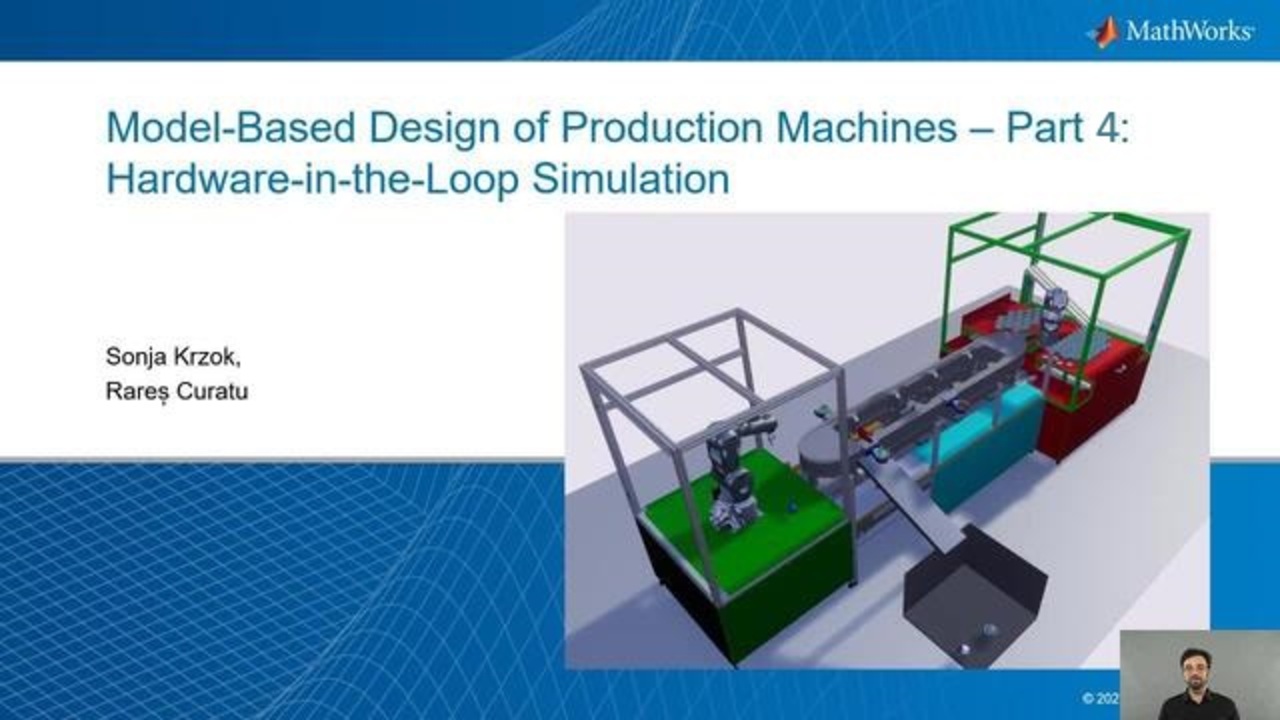
Model-Based Design of Production Machines – Part 4: Hardware-in-the-Loop Simulation

Hello, and welcome to the Model-Based Design of Production Machines webinar series. This is the fourth and final part of the series where we are going to talk about hardware-in-the-loop simulation. My name is Rares Curatu, and I'm an industry manager at MathWorks. Joining us today is my colleague Sonja Krzok from the application engineering department, who will guide you through the technical part.

Thank you, Rares for the introduction. My name is Sonja Krzok, and I'm a senior application engineer at MathWorks, Germany, with focus on real-time simulation and real-time testing. In this last session of this webinar series, we will talk about hardware loop simulations with MATLAB and Simulink, together with Speedgoat Real-Time Target Machines, and how you can test your PLCs.

This is the demo system model that we have been using throughout the webinar series. This model has five components that form an assembly line. The first robot is a Comau Racer V3. This robot picks up the cups and puts them in the shuttles. The second robot is a Mitsubishi RV-4F. The camera sensor in this robot's work cell detects the balls, and then this robot picks up the balls and places each of them in a separate cup.

The shuttle track moves four shuttles to robot 1, then to robot 2, and then to a conveyor belt before returning to robot 1. The conveyor belt carries the cups away from the track and into a container. The remaining non-moving model parts comprise the static machine frame which serves as the base for the assembly. It includes two work cells housing the robots, as well as the base for the sensor assembly.

In this webinar series, we have started with modeling, desktop simulation, code generation, and we are now going to address validation. We are following the typical steps that are taken when developing machinery software using model-based design. After simulating the plant and the desktop environment, designing and simulating the controller, and visualizing the simulations, we have shown the steps that you need to take in order to deploy the control algorithm on a Siemens PLC using Simulink PLC Coder and a Simatic Target for Simulink.

This way, the control algorithm that you have been developing in Simulink will be equivalent to the code running on the PLC. To continue the validation and verification of the software on the PLC, we will now deploy the simulation model of the plant on a real-time computer using Simulink Real-Time in a hardware-in-the-loop configuration. The real-time simulation will then communicate with the PLC through Profinet and also with a 3D visualization of the simulation.

On the screen, you now see the agenda for the entire webinar series and how the content is distributed throughout the series. In part 1, we have talked about how to import CAD models into MATLAB and then later use them in Simulink. In part 2, you have seen how to design supervisory logic for your PLCs using Stateflow. In part 3, we have deployed this logic to an industrial controller through code generation with Simulink PLC Coder.

The recordings of these three sessions are already available on mathworks.com. Today, in part 4, we round up the design process by testing the PLC in a hardware-in-the-loop simulation. During the presentation, if you have any questions, please enter them in the Q&A section. We will gladly answer them at the end of the presentation. Now, I would like to hand it over to Sonja for the technical content.

This is part 4 of the webinar series Model-Based Design of Production Machines. We will cover the topic, hardware-in-loop simulations. Let's have a look at the agenda first. We will start with a short introduction to hardware-loop testing with Simulink Real-Time and Speedgoat Real-Time Target Machines, which will help you to test industrial controls. And second, we will focus on the workflow.

During the presentation, we will answer the questions how to get from the desktop simulation to the real-time simulation, how to set up the Profinet communication to the PLC, but also the UDP communication, and how to deploy the plant model to the Real-Time Target Machine and run the simulation together with the 3D visualization. In the previous sessions, my colleagues covered the design and implementation phase.

Now, we're going to focus on the test and verification part through hardware-in-the-loop. And we will see how to ensure integration of validated software to avoid expensive hardware damages. For hardware-loop, we're using a dedicated real-time system. This will guarantee that our plant model is executed in real time and also the system is providing the different IO interfaces and industrial protocols to communicate with our device on the test, which is in our case, the PLC.

This will not only allow you to validate your control algorithm in the lab, but also to run automated tests in a closed loop environment. Also, you will be able in this setup to inject faults and test conditions without damaging the real hardware. So in the previous session, we already were at the model-in-loop simulation. This will be our starting point for the real-time simulation. To get there, let's have a look at our hardware-in-the-loop setup.

On the one hand, we have our target, the Siemens PLC. This is where our control algorithm is already deployed with the help of the PLC coder. Then, to run the plan simulation-- in our case, the robot's kinematics-- we're going to deploy the plant model to our Real-Time Target Machine, in that case a Speedgoat Baseline. And the third component is our host PC, which will run the visualization on the host PC.

The only hardware which is required is the Speedgoat Target machine. This will simulate the behavior of the plant and also provide all interfaces to which the PLC is connected. So this setup enables the user to test the PLC algorithm in various states and conditions already in the lab. With the hardware-loop simulation, you will achieve that the PC behaves as if connected to a real plant.

Before we have a closer look at the models, let's have a look at the hardware-loop setup in the lab. On the right side, we have the Siemens PLC where the controller is running. Next to it, we have the Speedgoat Real-Time Target machine, the Baseline, which is providing the Profinet interface to our PLC. On the host PC, we see all in the background a 3D animation running, and we are communicating from the host to the target through UDP.

And this will be the steps we are going to have to set up in the model. Split the model to the host PC and the Real-Time Target Machine, and establish the UDP in Profinet communication. Let's have a look at the model.

Our starting point is MATLAB Project, which is a great place to manage and organize all your required files, like the models we're going to use, the required configuration files, but also to collaborate with colleagues on the same project. You have the same setup, for example, having accessed that with those shortcuts to the most used files and models, but also to have already the source control there in place.

As mentioned before, our starting point will be the model-in-the-loop simulation. As we have learned in the previous sessions, the main parts of our simulation are the control algorithm itself for the actor motion, the plant model with the robot's kinematics, and third, the animation control for the 3D visualization. Now, for the hardware-loop simulation, we can use this model, modify it, and to make it able to run then also on the Speedgoat.

First of all, we can remove the control algorithm part, as this one is already deployed to the PLC. We're going to replace that part with the Profinet and UDP communication to exchange the data through host Real-Time Target Machine and PLC. Then second, we're going to split the model in two models. One model will be deployed to the Speedgoat-- this is our plant model with the robot's kinematics-- and second, the host model, which will run the visualization part.

Now on the left side, we see our host model with the animation control part and everything covered by the 3D Animation Toolbox. Now, to exchange the data between our hardware setup-- so between host Real-Time Target Machine and PLC-- we're leveraging here the UDP communication through the host target link which is already existing. So let's have a look on the input side.

So the UDP communication coming from the real-time target machine and then providing the data for the visualization-- therefore, we start with a UDP Receive block. And we are setting up here the local address from our host PC plus the remote address of the Speedgoat Baseline. On top of that, you have to define the data size. And after that, after having the data available, we need to unpack the data and then use it directly in our Simulink model.

In the Unpack block, we have to define the output port and data types and the different dimensions. OK. Same applies on the output side. There, we work with less signals we're going to share through the Speedgoat with the PSC. And same here, we're going to pick the data and send it through the host target communication.

Also here, we set the remote address and the local address and also defining the defined ports. OK, so this is our host model. As mentioned, it's running in your desktop simulation. What we can do to synchronize also the execution, we can leverage here the simulation pacing. So here, we have here the option that the simulation time is synchronized to the wall clock.

Now, coming to the Real-Time Model, on the one hand, we have here the plant model. So the robot's kinematics, as we have learned in the previous sessions, the setup exists of two robots. So we find here the kinematics of robot 1 and robot 2. And to exchange the data with the PLC, we have here the Profinet communication. This is a dedicated module on our Speedgoat Baseline. We will find the blocks for the communication and the speaker that will drive our library.

So let's have a look in our Simulink Library where you can find those blocks. So it's integrated directly in your Simulink Library browser that you find the Simulink Real-Time Speedgoat IO block set, and you have here access to all the different IO modules Speedgoat is offering. You select then the one dedicated on your system you're using. So in our case, it's the IO0752 for the Profinet communication. You always start with a Setup block for each module you're using.

Depending on the module you're working with this, can look a little bit different from module to module. For the Profinet communication, it means that we need to work with here the GSDML files. If you have an existing one from your devices, you can import it directly. Or, in our case, as our robots are programmed on our own, you can work also with a generic XML file which Speedgoat is providing.

So for the generic configuration, we have here the option then to configure the modules for the Profinet on our own by adding modules and submodules. Those configuration needs to match then also with the PLC configuration, based on the PC you're using. But here, you need to guarantee that the slots and sub slots and sub module are matching so you're able to exchange data. OK.

On the other hand, we have also here then an on top a Network Status block. So if in case of, for example, a misconfiguration or an problem on the network, you can also track the status directly here with a Status block. For all the Speedgoat IO block sets, you also have the quite detailed documentation, also with, for example, usage nodes, which are explaining really in detail how to configure the different modules, how to set up those IOs, and the communication to get started.

You also find the different examples of loopback examples so you also can test the setup on its own without additional hardware. So that's a great place, great resource to get started if a certain module is new to you. So that's on the one hand for the generic setting. So we have set up everything here. Now, to read and write the data on the Profinet bus, we're working here with the Send and Receive block.

So on the one hand, we're sending a few signals from our simulation. Therefore, we have the byte reversal to match then the data format. Based on this record system, we pack the data, and then we send the data on the bus. And here, we can automatically retrieve the configuration based on what is set in the Configuration block, so nothing else than retrieving your configuration you have already defined. And the same applies then on the input side.

So on the receive side, let's have a look on the Block Mask. You're referring here to the module ID that would be different than if you would use the same module several times. Then you would work with different module IDs. If you have the same module only one time, it's module ID 1. And you can also change the sample time in the IO blocks directly if you want to-- if you want to have a different than the execution time, for example, of the plant model.

And also here, we retrieve the configuration automatically. Based on that, we have the Send and Receive blocks, the Byte Pack and Unpack, and then we have the blocks directly integrated in our Simulink model to exchange the data directly. So that's it basically for the modeling part. Now, to deploy the model to the real time target machine compared to executing on the host machine we have here the option to go through Apps and search for Real-Time.

And with this one click, our model will be configured and directly to be able to deploy it to a Real-Time Target Machine and no other steps in between. Assuming you have done the configuration here, let's have a look in the model settings. You will see here in code generation that Simulink Real-Time is set as system target file. And that's one of the mandatory settings to be able to generate the Real-Time application.

As soon as you went or done those steps, you will find here this new tab called Real-Time. And here, we can basically go from the left to the right. So the first step is that you select your Real-Time Target Machine, and you connect to your target. So we're establishing the host target connection here. And then, we can go to the right and click Run on Target, which is like the one-click option to start the process.

If I click on that little button, you will see that there are several steps which will be executed then automatically. First step is to build the real-time application from our Simulink model, deploy then to the Real-Time Target Machine, and then start the application. And you can execute those steps one by one or Run a Target is like the one-click option.

When you trigger the process build application, you have different ways how to follow the process. For example, in the diagnostic views, we will see in a second. But also, I will show you an option through SSH. Now, to run both in co-simulation, I can start the process now here with Run from both model. So the simulation is started. On the one hand, we have now the visualization here. Let's change the view.

On our setup with the robot, and the conveyor belt, the cups, and the balls so we see the 3D animation is running. We see here the execution time from the host model. We see now also in parallel for debugging purposes, we have the option through SSH how then our Real-Time Target is doing. So let's open that in parallel. I have here SSH session.

So I can log into the target, and I can open a status monitor, for example. And I get there the information of how my target is configured, but also here the state that the Real-Time Model is running, the execution time-- the task execution time-- but also here log output. But also on the host, we can have a look at our Real-Time Target Machine with the help of the Algorithm Explorer.

So we see here, we're connected to the Baseline. There's a Real-Time Model running. We see it from there. We see also here the execution time directly. And, for example, we have here the option to visualize the task execution time with this monitor, but also having access to the System Log Viewer where we get, for example, information about the Profinet communication.

And from there, you would be also able to load the applications that stop it having access to the different parameters and signals, OK. If I stop the simulation, we can also have a look at the signals, which are available in the Simulation Data Inspector. And that's basically the same tool you already know from the desktop simulation, which you can use also for the real-time simulation.

So if you have-- so having a look at the model, we see here the Data Inspector of our Real-Time Model that there's data available. We see here from the current run-- run 14 and 15-- our host model, but also the Real-Time Model with the addition at Baseline. So we know that it has been executed at a dedicated Real-Time Target Machine.

And from there, we can have a look at our different signals, for example, the ball instance, which is just a counter for all the different-- for the number of balls which are detected, for example. But we can also visualize, for example, the different shuttles and their positions. And the same applies for the host simulation part and the thickness we have selected for streaming.

With this, we are already at the end of our session for hardware-loop in simulation and testing. To wrap up, I would quickly like to highlight three end points. First, I hope you could see how hardware-loop testing allows you to include real signals and communication interfaces. But also, how you can verify and validate your controller on real environments and different events and conditions. And that this finally allows you to test your PLC in a safe and deterministic environment. Thank you for your time and your attention.

Thank you, Sonja. Validating PLC code with agile testing can sure make any acceptance test go a lot easier. This is the end of today's presentation. But before we end today's session, we will be answering your questions. So if you haven't already, please type your questions in the Q&A section. This was the last webinar of the four part series. The recording will be made available together with the first three.

If you plan to attend Forum Industria Digitale in Italy, SPS in Germany, or the Precision Fair in the Netherlands this November, we will be happy to meet you there in person and talk about your projects. In the meanwhile, if you want to take a look at what else industrial automation and machinery engineers are using MATLAB and Simulink for, please visit mathworks.com/industrial-automation-machinery. Thank you for your attention and for your interest. And now let's take a look at the Q&A section.