How to Perform SLAM on Rough Terrains

Welcome to this tutorial about performing SLAM for vehicles on rough terrains. This is part of the MathWorks Autonomous Construction Vehicle series. My name is Bojian. I am an engineer at MathWorks, working on robots and autonomous systems. SLAM is short for Simultaneous Localization And Mapping, and is commonly used for autonomous vehicles.

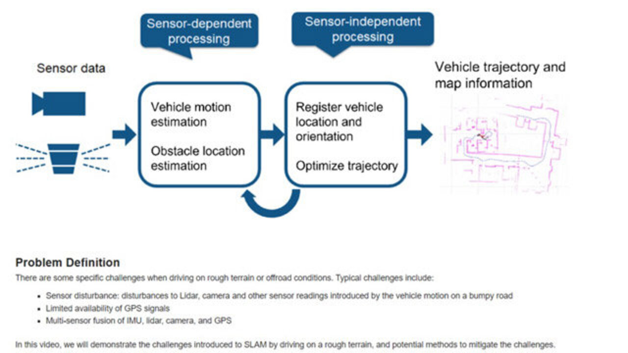
There are some specific challenges when driving on rough terrain or off-road conditions. Typical challenges include the following-- sensor disturbance-- the vehicle motion on a bumpy road introduces disturbances to lidar camera and other sensor readings. In addition, when we are driving in clustered environments, we may have limited availability of GPS signals. Moreover, we often need to fuse multiple sensors to get more accurate SLAM results and face the challenge of effective and accurate sensor fusion.

In this video, we'll demonstrate the challenges introduced to SLAM by driving on rough terrain, and potential methods to mitigate the challenges. The input to the problem is a ROS bag that contains the lidar, camera, MU, and odometry for the duration of a vehicle driving through the construction site. We collected ROS data from the third-party game engine scenario. The output is a 3D map that should resemble the construction site. The goal is to minimize the discrepancy between the output map and the ground truth.

The following of this live script demonstrate the process. First of all, we load the data we need. We select the ROS bag, convert the data to MATLAB timetables, and process the lidar data. In this example, we use a lidar SLAM algorithm. This figure shows the output of a lidar sensor at one measurement. It is a collection of points in 3D space and that is the point cloud.

We then use the point clouds to build a map following two steps. The first step is aligning successive lidar scans with respect to the first scan. The second step is to combine all align scans and merge all point clouds to generate a complete map. This process is called point cloud registration.

In this section, we define a list of parameters for this purpose. I would like to point out two parameters that are going to significantly impact the results-- random sample ratio and great step. Before we get into the details of the algorithm, I would like to present the effects of changing random sample ratio and the result of map construction. In our example, when we use a random sample ratio of 0.3, the algorithm fails soon after we start building the map. As we progressively increase the value, we get better maps.

In the next section, we tune the parameters to search for loop closure. A loop closure is when the vehicle visits and recognizes a previously mapped duration. A loop closure query-- the robot looks around itself, compares this region with visited places, and determines if the current region has been visited. Due to the uncertainty in real-world sensing, the trajectory and map are not ground truth, but rather our most confident estimate. The SLAM algorithm uses the loop closure information to reduce the uncertainty in mapping and increase confidence in the estimate. For brevity of this script, we put all variable initialization in one single function, detailed in the following bullet points.

Now we're ready for trajectory estimation and refinement. The algorithm has the following steps-- point cloud filtering, point cloud downsampling, point cloud registration, loop closure query, and post-graph optimization.

In the first step of point cloud filtering, we're most interested in mapping out the buildings, their walls, and corners. To focus on these, we will remove the ground and sky.

The second step is point cloud downsampling. In our example, a random downsampling improves the speed and accuracy of the point cloud registration algorithm.

In the third step of point cloud registration, an algorithm aligns the scans and finds the relative position of all future scans with respect to the first one. Thus, we can merge the point clouds from all scans to construct the complete map.

We mentioned the next step, loop closure query, when defining its parameters. The loop closure search is performed by matching the current scan with the previous scans within the radius. When we know there is low drift in lidar odometry, it is sufficient to search within a small radius around the robot. However, searching against a larger radius is necessary when there is a high drift, and the search becomes time consuming.

The last step is post-graph optimization. After a loop closure is detected, we use this information to do an optimization on the complete trajectory, in order to reduce the effects of uncertainty in lidar sensing and increase the confidence in the estimated trajectory and the generated map.

Running this example will build the map in this figure. The occupancy map is color coded by height, and the vehicle's trajectory is shown by the blue line. Now, if we rotate the map in 3D, we can see there are misalignments in the z direction. This is likely to occur when the ground is uneven and there are a lot of noises in the z direction.

Here is the ground truth map, in the same orientation, for comparison. But how can we improve the performance of this lidar SLAM? We will look at three sets of parameters and their effects on map construction.

The first parameter specifies downsampling. It is a parameter between 0 and 1. A higher value indicates sparser point clouds. Four subfigures are generated, using a random sample ratio of 4 values respectively. When we use a value of 0.3, the map construction fills soon after start. When we increase downsampling, the performance gets progressively better. A smaller value is suggested when you need a very dense occupancy map, and the odometry is very accurate. In this example, a higher value of downsampling is recommended.

The second parameter we'll look at is reg gridStep. We vary the parameter from 1.5 to 3.5, in a step of 1, and 2.5 seems to perform best.

The third set of parameters are related to the closure detection. If we enlarge the closure search space using the following parameter values, we can detect one loop closure. This figure shows the built map, before and after post-graph optimization.

Now it's your turn. We encourage you to play with the parameters and see how much you can further improve this SLAM result, to make it closer to the ground truth.