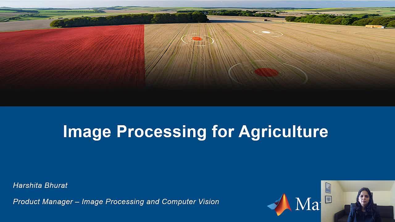
Image Processing in Agriculture
From the series: MATLAB for Agtech Video Series
The agricultural sector is undergoing a data-driven transformation. There is increased adoption of technologies like remote sensing, manned or unmanned aircrafts, and terrestrial sensors for precision agriculture, and the use of data analytics and smart farming technologies is improving yield and profitability.
Highlights:
- Hyperspectral image processing with MATLAB®
- Interactive analysis with the Hyperspectral Viewer app
- Aerial lidar data processing for terrain classification and vegetation detection
Recorded: 20 Apr 2021
Hello, everyone. My name is Harshita Bhurat. I'm the product manager of image processing and computer vision systems at The MathWorks. Welcome to today's session on image processing for agriculture.
Our customers have been using our tools and agriculture and environment monitoring for quite a few years now. Today, I'm going to talk about a couple of these use cases. The first one here is NASA. So NASA's Stennis Space Center developed ForWarn which is an environmental monitoring and assessment system that detects and tracks changes in forest vegetation nationwide.
So what ForWarn does is it analyzes multispectral satellite imagery to identify almost in near real time potential for disturbances that are caused by insects, droughts, storms, wildfires, et cetera. And the system also enables users to view all of these changes on a map.
NASA engineers use MATLAB to develop and deploy this ForWarn software while working with other government agency partners. At MATLAB, these engineers produced prototypes and built products much faster than they would have with traditional programming languages such as C, which they were working with before. So this quick turnaround time helped them demonstrate new capabilities quicker and faster to their customers. They specifically found working with multidimensional data very easy in MATLAB. This works well for analyzing satellite imagery, and it saved them years of development time.
Not only big organizations such as NASA but a lot of startups and small organizations have benefited from using our tools as well. Here, you see Gamaya. It's a Swiss precision agriculture company that captures hyperspectral images with satellites and custom drones. They use all of this data along with data from weather stations and ground sensors to detect specific traits within the plants.
In many cases, the undesirable plants or weeds can look very similar to the actual crop, specifically in the RGB color space where these differences are not easily perceived by the human eye. Hyperspectral images, on the other hand, use extra bands of light to capture these specific traits. So now, the combination of spectral and morphological characteristics can help easily differentiate a weed from a crop plant.
IntelinAir is a US-based precision agriculture company. They specialize in aerial imagery and analytics. They use manned airplanes to get images of the fields and then leverage a combination of visible, near infrared, and thermal cameras for all of their analysis. They capture images throughout the growing season. With these images, the farmers can either get a snap shot at any given time or they can gather trend data for longer term planning. So this helps alert the farmers to problems so that they know when they need to take action.
As you can imagine, the agricultural sector is undergoing a data-driven transformation. Data analytics and smart farming technologies-- they're being used to improve both the yield and the profitability from all of the farms. We are also seeing increased adoption of technologies like remote sensing, aircrafts, both manned and more unmanned aircrafts, and terrestrial sensors for precision agriculture.
In the past few years, we have seen significant adoption of hyperspectral imaging activities in agriculture. This adoption is mainly due to the evolution of sense of design, and hence, a resulting in availability of low-cost hyperspectral cameras. As a result, now, there is a growing need for processing and analyzing these hyperspectral images, and also applying AI and deep learning techniques on these images for smarter and efficient farming techniques.
These hyperspectral cameras, along with other sensors such as thermal cameras and lidar sensors, are then mounted on unmanned or manned aircrafts and drones to capture images of the terrain. This is driving the need for autonomous navigation and mapping techniques as well.
Very soon, we will see the convergence of hyperspectral imaging, computer vision, image processing, and autonomous applications. Hence, for today's agenda, I'm going to go through two topics. The first is vegetation analysis using hyperspectral image processing. I will go over a few examples to show how to do that easily and effectively in MATLAB. The second is 3D mapping of aerial radar data. This can be then used for terrain classification and vegetation identification in agriculture applications.
Let's start with hyperspectral image processing. Before we drill into hyperspectral image analysis, let's just briefly touch on what we can do for traditional image processing in MATLAB today. For a long time, MATLAB has provided a very large, and it's a growing database, of built-in algorithms, functions, and libraries for all kinds of image processing techniques like filtering, segmentation, de-noising, adjusting image and density to get more out of the image, registration, even detecting objects from an image, et cetera.
Over the last few years, MATLAB has introduced a large number of apps to support a bunch of these image processing techniques. So what are apps? Apps are interactive GUIs. So these apps help you explore various algorithms. And once you've established a workflow by finding an algorithm that works best for you, you can then use these apps to also generate functions or MATLAB code from it. You can then use these functions in MATLAB code in bigger systems for iterative workflows.
Today, I'm going to show you some of the apps that I used for creating and analyzing masks. The first one here is the Color Thresholder. The Color Thresholder manipulates color components of an image based on different color space. You can see the image here white clouds representing the image in four color spaces-- the RGB, the HSV, YVBCR, and LAB.
For color-based segmentation, you can select the color space that provides the best color separation for your image. You can use that to create a mask. To segment the image in another color space, you can click the new color space and try a different color space before you achieve a segmentation that meets the needs. Using this app, you can explore between different spaces and create a segmentation mask for a color image.
Next, here, you see the Image Segmenter app. With this Image Segmenter app, you can perform different morphological and segmentation techniques interactively. Using the Graph Cut technique, you can select the foreground and background and then use the Freehand ROI drawing to fine tune the results. can also use Flood Fill and invert mask mask to achieve a similar segmentation result.
Once you have multiple segmentation sessions, you can now compare the results visually and pick the one with the most suitable result. Once you've landed on a segmentation technique that works for you, you can either export these images, or you can generate a function or MATLAB code from it.
Once you have a foreground mask, you can perform additional processing based on region properties. The Region Analyzer app enabled a quick and interactive phase of exploring and filtering out the connected components within an image based on the geometrical properties. In this app, for example, we're using area to filter out regions smaller than certain chips in the image. The table on the right shows all of the properties of the connected components, and then you can use those to explore different properties that may be useful in your algorithm.
The next is the Labeling app. In this video, you will see how the label apps provide automation capabilities to accelerate the labeling process. These data labeling apps work on both images as well as videos. You can use techniques such as semantic segmentation. In it, regions of the image are classified, and then that classification is automatically applied through every frame of the video. As with other apps, the labeling apps also generate code through use.
The Image Labeler also supports very big or what we call blocked images. This allows you to label very large images that do not fit into memory. And you can do this interactively. You don't have to worry about extracting patches, labeling each patch, and reconstructing the image. Instead, you can interactively move around the image and label the different parts of it.
We are all familiar with RGB images from a regular camera that censors three wavelengths. But hyperspectral senses, on the other hand, collect information as a set of images. Each image represents a narrow wavelength range of the electromagnetic spectrum. This is also known as the spectral band.
All of these individual images are then combined to form a three-dimensional hyperspectral data cube. Each wavelength captures a different property from the scene, such as one may capture color, another intensity. Some might capture material properties. Some might capture presence of moisture. Some might capture the vegetation, et cetera. The hyperspectral cube can then be processed and analyzed to make sense of all of the content of the scene.
To work with these hyperspectral data cubes, MATLAB has a hyperspectral image processing library that provides functions and tools for hyperspectral image processing as well as visualization. You can use these functions to read, write, and process hyperspectral data.
This hyperspectral image processing library supports a variety of file formats captured from different hyperspectral imaging sensors. The library also presents a set of algorithms for end-member extraction, abundance map estimation, atmospheric correction, dimensionality reduction, and so on. The library also contains a hyperspectral viewer app which helps read and visualize hyperspectral data.
This here is the hyperspectral viewer app. In this app, you can import any hyperspectral cube and analyze any particular band of that cube, along with the band's contrast stretch or dynamic range. We will import the Jasper Ridge data set into this app. The first thing that the app displays is the false color composite. The false color composite visualizes wavelengths that the human eye cannot see.
The top of the panel identifies the type of the color image. Here, for example, false color. And also list the bands that the app used to form it. Here, you see 145, 99, and 19. The app supports three types of color composite renditions. False color, RGB, and the color infrared CR out of the box.
For visualization, you can change these bands by clicking and dragging the handle of the band indicator here at the bottom in the spectrum plot. You can also create spectral profile lots of pixels or regions. You can use the neighborhood size slider there to specify the region size.
For example, in the given image, you can have four points selected representing a particular type of data. For example, water, vegetation, road, and land. It can be helpful to view all of the color composite images because each one of them uses different bands and can highlight different spectral details of the image. You can see how this can help in the interpretability of the overall data.
There is a generalized workflow for processing hyperspectral images. You have a hyperspectral data in the form of a data cube. Then you either pass the data directly for analysis and algorithm development, or you perform some preprocessing to remove artifacts from images. Like, for example, smile correction, atmospheric correction, radiometric calibration, and denoising of images.
If you already have corrected data, you can skip the preprocessing part and directly work on processed data for algorithm development. This algorithm development is basically working on anything like material identification, object detection, classification, so on and so forth. We will look at some of these workflows in a little bit of detail.
This here is the preprocessing step for hyperspectral imaging. No matter what workflow you choose, like classification or spectral unmixing, et cetera, this is a common step. As we saw before, it's also optional. You don't always have to do preprocessing. And this preprocessing includes steps like atmospheric correction, selecting bands, or, in some cases, also reducing dimensions.
Spectral unmixing is really a source separation problem. Here, the goal is to recover the spectral signatures of the pure materials in the scene, like, as we saw, land, or water, or road, et cetera. These are also called end members. And in some cases, we have to estimate the proportions of each of these end members in each pixel. That's called abundance map estimation.
The next workflow is classification. Classification allows us to process the entire hyperspectral cube and determine different end members or different materials are present. For example, identifying rods in an image, or identifying vegetation in an image, or identifying water bodies in an image.
Spectral matching workflows include matching techniques that are used to match class spectra with an ideal spectral. This is used for several applications such as identifying of crop types, identifying specific plant species, or, for example, for mineral exploration. This is one of the very widely used workflows and commonly requested workflows from our customers, and this is what we are going to drill more into today.
MATLAB provides a built-in function for spectral matching. This function can use spectral signatures either from a hypercube or from a public spectral library. On the slide here, you see three use cases for spectral matching. First, spectral matching can be used for material classification. As you can see in this, the material in the image has been classified as sea water, tree, concrete, et cetera.
The second use case is for locating a material in an image. Here, we have detected roof material in a given image. The third use case is to identify the name of the material. For example, here, you can see members have been specifically classified as limestone, concrete, asphalt, et cetera.
I'm going to show you a MATLAB example for one of these. This workflow shows how to detect and on target in an hyperspectral image by using the spectral matching method. In this example, we will use the spectral matching method called Sam, also which stands for Spectral Angle Mapper, to detect manmade roofing materials.
The pure spectral signature of this roofing material is read from the ECOSTRESS-- library. This spectral signature is used as a reference spectrum for spectral matching. And each and every pixel of the data cube is then compared with this reference spectrum.
The best matching pixel to that reference spectrum is classified as belonging to the target group material. And that helps in identifying the entire group target in the hyperspectral image. Now, let's see that workflow in MATLAB. Here is an example to detect manmade roofing materials, which we can also call the target in a hyperspectral image.
First, we read the hyperspectral data. In this case, it's the top of the buildings. Then we read the spectral information corresponding to the roofing material from the ECOSTRESS spectral library. Here, we're reading the wavelength and reflectance values stored in the library which contain the reference spectrum. You can also visualize the reference spectrum from the ECOSTRESS library.
Now, we can estimate the spectral similarity between the reference spectrum and the data cube by using the spectral match function. By default, the function here in MATLAB uses the Spectral Angles Mapper, also known as SAM method. The output that you see here is a score map. The score map signifies the matching between each pixel spectrum and the reference spectrum. Lower value of the SAM score represents better matching. We can then leverage thresholding to spatially localize the target region in the input data.
So here, we are performing thresholding to detect the target region with maximum spectral similarity. And then on the right here, we're over the threshold at image onto the hyperspectral data. We can then validate the obtained target detection results by comparing it with the ground truth, which is also taken from the Pavia University data set. On applying the same spectrum matching algorithm to our Jasper Ridge data set, we get this output. As you can see that the vegetation identification using the SAM function is very, very close to the ground truth that's provided in the data set.
This next workflow expands the previous target detection workflow and applies it for image classification. Here, now, the data set contains foreign members. So instead of reading one spectral file, we read spectral files related to each of those four end members. For example, the spectral file related to water, related to vegetation, to soil, and to concrete, from, again, the same ECOSTRESS spectral library.
We can compute the SAM spectral matching score between the spectrum of each test pixel and the pure spectrum read from the spectral library. We generate a score map for each of the end members. So now, instead of one score map, we have an array of score maps.
For classifying the regions, we use the minimum score criteria and assign a class label for each pixel in the test data. The resulting output image is the classification map for our Jasper Ridge data. And you can see every pixel in that image classified into one of the five categories for sea water, tree, concrete, et cetera.
The hyperspectral library provides a set of 15 hyperspectral indexes. These indexes help users analyze vegetation and other materials. They cover different aspects of the image, such as greenness, the nitrogen content, crop residue, and also other miscellaneous objects like water, building material, burn areas, et cetera.
On the slide, you see the analysis of the water region using the NDWI, which is the Normalized Difference Water Index. The bottom image is the ground truth image in which the water is shown in blue. In the top image, you can see that we have almost accurately identified the water region, and it's overlaid in yellow on top of the original image.
One such very popular and widely used hyperspectral index is the NDVI, which stands for Normalized Different Vegetation Index. The NDVI map of a hyperspectral data set indicates the density of vegetation in various regions of the hyperspectral data. NDVI is a simple graphical indicator that can be used to analyze whether the target contains live green vegetation or not.
You can compute the NDVI value for each pixel in the data cube by using the NDVI function. The function outputs are to the image in which the value of each pixel is the NDVI value for the corresponding pixel in the hyperspectral data cube. You can then segment the desired vegetation by performing a simple thresholding of these NDVI values.
In this example, here, you can see that you can interactively select and change the threshold values to identify different regions in the hyperspectral data cube. This thresholding is based on their NDVI values. Based on these values, you can identify if the vegetation in a region is dense, sparse, moderate, or does not exist at all.
You can use more than one of the spectral indices from different categories for vegetation health monitoring. Here, we are using four indices to better understand the status of our crops. The first one is the PRI, which is the Photochemical Reflective Index. This index talks about the light use efficiency of the vegetation.
The next index is SR. Which stands for Simple Ratio. It is an indicator of greenness of the vegetation. MSI, the Moisture Stress Index, is a good indicator of leaf water content. And MCRI, or Modified Chlorophyll Absorption Ratio Index, indicates the relative abundance of chlorophyll in the vegetation.
Here, what you see on the slide is output of applying all of the four hyperspectral indices to a hyperspectral data cube and identify stressed or unhealthy vegetation. Stressed vegetation is vegetation with low sunlight, low moisture, and low chlorophyll content. This is the one that you see overladen in yellow on the hyperspectral image.
That was just one label to identify stressed vegetation. We could use multiple labels to further classify and identify vegetation as healthy, stressed, or lack of vegetation at all. Now, if you're applying the same algorithm to the Indian Pine point data set. And finally, the same applies to our Jasper Ridge data set as well.
The hyperspectral library also provides a workflow and examples to show how to classify hyperspectral images using deep learning networks, such as, for example, the CSCNN, which is the Custom Spectral Convolutional Neural Network. CSCNN learns to classify about 16 types of vegetation and terrain based on unique spectral signatures of each of those materials.
Here on the slide, you see an example of a hybrid spectral net. Essentially, for any of the deep learning networks processing hyperspectral images, we can split it into these five steps. The first is reading the hyperspectral image and the ground truth. Then you reduce the spectral dimension of the input data using PCA or any other algorithms.
Then, you split the data into patches and label the center pixel of every patch. Then you train the network and finally create a deep learning model out of it. Today, I'm not going to go into details of the examples, but I can show you some of the outputs using this network.
Here, this first image is from the Indian Pine data set, and using image classification with CSCNN, you can see that the predicted classification is very, very close or almost identical to the ground truth classification provided in the Indian Pine data set. This is applying the hyperspectral image classification on our Pavia data set. Again, the ground truth is very, very close to the predictive classification. You can find all of these reference examples in our documentation.
That concludes the first section of today's presentation-- the vegetation analysis using hyperspectral image processing. The next part of the presentation goes through a workflow for autonomous navigation and mapping. I will show you an example for 3D mapping using aerial radar data.
Lidar sensors are everywhere. With lidar cameras getting smaller and cheaper, we are seeing a large adoption of this technology, specifically mounted on autonomous systems like UAVs drones, autonomously driving tractors, and ground vehicles. So MATLAB provides the Lidar Toolbox which contains algorithms, functions, and apps for designing, analyzing, and testing all of these Lidar processing systems.
Here on the slide, you can see all of the categories of functions that are supported in the lidar toolbox. The functions range from apps for lidar camera calibration to being able to read lidar data, either from various file formats or directly from the lidar sensors, to support for deep learning with lidar labeling apps. The Lidar Toolbox provides reference examples for perception and navigation workflows.
Today, we will specifically focus on 3D mapping using aerial lidar data and use an example to implement SLAM, our Simultaneous Localization And Mapping, on onpoint cloud data which was collected by a lidar sensor that's mounted on a UAB. This is what the workflow looks like. First, we read or load the point cloud data into MATLAB. Then we preprocess this lidar data and register the point clouds.
Finally, we implement post-graph optimization to correct the drifts that may have occurred during the point lab registration stuff and build a complete map of the surrounding area. Let's begin by reading in the lidar data. MATLAB provides the flexibility to import point cloud data from various file formats like PCD, PLY, PCAP, and so on. You can also directly stream data from the Velodyne lidar sensors or read point cloud data from ROS bags, which are very popular in autonomous systems.
This function shows how to read and process lidar data in MATLAB. We use the Velodyne reader function to read in the PCAP file into MATLAB. We then use the PC player to visualize the point clouds. PC player is a very convenient tool. You cannot only visualize but also analyze the point clouds. You can Zoom in. You can zoom out, rotate, pan. You can also use data types to get details of any specific points in the point cloud.
In MATLAB, the point cloud data is stored as a point cloud object. It includes all properties associated with point clouds, such as location, color, intensity, count, and x, y, z limits. On these point clouds objects, you can perform the following functions. You can find nearest neighbors. You can find points in any specific region of interest. You can remove invalid points from the point cloud and select points using specific indexes.
Now that we have collected our point cloud data, we can perform some basic preprocessing. For example, you can use PCD noise function to remove noise from the point cloud based on a predefined threshold. You can then use PC downsample to downsample point cloud without compromising its structure.
As you can see here, the number of points and the points that have reduced from 34,000 to about 26,000. And there is no change in structure of the point clouds. You can refer to the Lidar Toolbox documentation to find more preprocessing functions.
The next step is to perform feature-based point cloud registration to create a 3D map of the environment. Point cloud registration is the process of stitching multiple point clouds to form a combined bigger point cloud. If you have point cloud data and accurate post information for each instance, we can use the post information to stitch the point clouds.
But sometimes, this is not the case. In most cases, the post information is incorrect and inaccurate. So we'll show an example to use only point cloud data to create the 3D map of the environment. We are going to see that in MATLAB.
We begin with reading two point clouds and performing some basic preprocessing like ground removal and downsampling. We then extract the FPFH features from both the point clouds and match the features using built-in functions in MATLAB.
Here, we can see the two point clouds, one in red and one in blue, and the match features are connected by the yellow lines. Next, we will use these match features to estimate geometry transformation between the two point clouds. This function gives you the rigid transmission between the two point clouds. The PCL line function then aligns the point cloud based on the rigid transmission matrix from the previous step.
For a series of point clouds, we go through the steps iteratively of preprocessing, extracting, matching FPFH descriptors, estimating transformation, and aligning the point clouds. Then after we're done with point of registration we finally apply post-graph optimization to correct the drifts from registration and use it to build an accurate 3D map. The post-graph optimization will not be covered in the talk today, but we can point you to a material that you can refer to do that accurately. Here is a final output map after post-graph optimization. As you can see that it's very identical to the ground truth map.
Now that you have the 3D map from the previous step, you can use that 3D map to perform semantic segmentation of the lidar data. Here, you can see the point cloud that is overlaid with all of the other semantic labels such as cars, trucks, vegetation, pools, buildings, et cetera.
You can also use the 3D map to segment and classify terrain in aerial lidar data. Here, you can see the terrain classified as ground, building, and vegetation. There is an example in the documentation that contains lidar data captured by an airborne lidar system. This lidar data is fed as input.
Then the point clouds are classified into first, ground, and non-ground points, and then subsequently into building and vegetation points based on specific features. This figure here provides an overview of the process. As I mentioned, you can find both these examples and workflows, and you can refer to them in the MATLAB documentation.
Today, we developed an algorithm for vegetation analysis using hyperspectral image processing. We also designed algorithms for 3D mapping using aerial lidar data. However, these algorithms have to be incorporated into a larger system to be useful. For deployment, we have a unique cogeneration framework that allows algorithms that are developed in MATLAB to be deployed anywhere without having to rewrite the original algorithm. This gives you the ability to test and deploy the entire system and not just the algorithm itself.
MATLAB enables you to deploy your algorithms, workflows, deep learning networks, et cetera, from a single source in MATLAB onto various embedded hardware platforms. They could be MPDR GPUs, Intel and arm CPUs, or Xilinx and Intel SSCs and FPGAs. With the help of the MatWorks coders, you can explore and target embedded hardware easily.
MATLAB can generate native optimized code for multiple frameworks, so this gives you the flexibility to deploy to lightweight, low-power embedded devices such as mobile phones and iPads, low-cost rapid prototyping ports such as Raspberry Pi, and even on edge-based IoT applications such as sensors and controllers on a machine in a factory.
So here are the key takeaways from today's talk. MATLAB provide interactive and easy-to-use apps to help explore, iterate, and automate your workflows. MATLAB also provides built-in functions and algorithms for visualizing, analyzing, and processing hyperspectral images. You have workflows unexampled to construct and update 3D maps from lidar sensors that are mounted on autonomous systems.
Here are the three toolboxes that I touched on and the algorithms that we talked about today. The Image Processing toolbox, the Computer Vision toolbox, and the Lidar toolbox. That brings us to the end of our presentation. And now, I can answer any questions that you might have.
Featured Product
Image Processing Toolbox


Select a Web Site
Choose a web site to get translated content where available and see local events and offers. Based on your location, we recommend that you select: United States.
You can also select a web site from the following list
Americas
- América Latina (Español)
- Canada (English)
- United States (English)
Europe
- Belgium (English)
- Denmark (English)
- Deutschland (Deutsch)
- España (Español)
- Finland (English)
- France (Français)
- Ireland (English)
- Italia (Italiano)
- Luxembourg (English)
- Netherlands (English)
- Norway (English)
- Österreich (Deutsch)
- Portugal (English)
- Sweden (English)
- Switzerland
- United Kingdom (English)