Mathematics and Matrices in MATLAB
Learn how to perform quick mathematical analyses and matrix operations with MATLAB® to get quantitative insights from your data.
Published: 9 Nov 2020
Hello, and welcome to today's session on mathematics and matrices. I'm Lawrence, an application engineer at MathWorks. Here's our agenda for today. Today's session is broken down into two parts. In the first part, we'll be looking at basics of mathematics and matrices. In the second part, we'll be looking at how to identify trends and fit distributions. For working through the second part, we'll be using an example using trading using regression models. We'll be closing the session with a trading strategy fit using several regression models using zero lines of code. The app is called Regression Learner, and you'll be looking at how we could use this.
Here's the data that we'll be working with today. We'll be looking at time series of stocks. Let's go to the first demo. Before we get into the demo, let's have a look at the data that we'll be working with. So here we have the stock names. We have 30 of these stocks. And we have prices that goes from 4th of January, 2018 until 27th of December, 2019. Let's go ahead and bring this data completely into MATLAB.
My first script here is called basics. Let's go ahead and start with that. So for reading an Excel file into MATLAB, the function that I'm using here is readTimetable. So it reads this Excel file in the format of a timetable. Let's go ahead and execute that.
Now we can see that the entire Excel file has been loaded into this variable called prices, so I can scroll down to the end and see that the last date that I would have is 27th of December, 2019. If I hover over these column names of, let's say for example-- the first column name is KMI. I can get this arrow, upon clicking which, I have some interactivity. I could sort largest to smallest or smallest to largest. If I go ahead and choose to sort this entire table by the values that is there in the column KMI, I could do that by setting sort smallest to largest, in which case, the code would be that.
If this is my intention to preserve this, I could go ahead and say Update Code, which case, that line gets added to this code over here. Let's keep the way that we imported the data, sort oldest to newest, that's how we saw it, update code. And you can see that second line gets added to the code as well.
That said, if I open this variable in variable editor by right-clicking on that variable and asking MATLAB to open prices, it opens prices in variable editor. Over here, I could click on time and on, let's say, any of these columns, go ahead to plot, click on Plot, and quickly get an idea of what the time series look like. The corresponding code has been written out by MATLAB. And I've got the x-axis, which is a date time axis. If I go ahead and zoom in, notice how the x-axis gets automatically updated. And based on the granularity that you have for your data, you could go down to nanosecond-level precision.
To access a subset of data, so in our timetable, we have NKE, AAPL over here, and WMT over here. Let's say we want to pull out just these three columns from our timetable. We could do that by using this notation. So we specify the variable that we're interested in. Within brackets, we specify, we call an operator for accessing all the rows, and within square brackets, we specify what columns we're interested in.
So if I go ahead and execute that by using the shortcut Control-Enter, you can see that I've created a subset of just Nike, Apple, and Walmart. I could also say get a column based on the column number. So for example, if I'm interested in the second column, so that's, 1, 2, TXN, I could specify get me all the rows and the second column and then have that. So I get a subset of just the second column.
I could also specify to get columns based on column numbers. So in this case, if I want to get Apple, Walmart, and Nike, I could also use the column numbers 6, 7, and 16, in which case, I get the same output as here. Nike, Apple, and Walmart. So here, I see that the order is inverted. So if I want it in the same order, I can flip these numbers over here, 7 and 16, in which case, I get the same order as before. To store the subset into a variable, I set that subset into a variable by using the equal operator.
Now thus far, we were taking a subset based on columns. Now what if you're interested in using a subset of the rows? So for doing that, we are going to use dateTime vector. So let's see, I'm interested in only rows between 10th of January, 2018 and 20th of January, 2018. So it should give me all the rows between 10 and 19.
For doing that, I'm going to be using a vector called dateTime vector. And how am I doing that? Let's just take this command, this piece of code, into the command window. So what I've done over here is I've created a dateTime vector. So what is dateTime? So let's start with that. So dateTime, if I specify a date, 01, which is the month and 10th, that gives me the date, which is 10th of January, 2018.
And if I want all the days between the 10th of January until the 20th, I could do that by specifying the colon operator, the starting date and the ending date separated by the colon operator. So when I do that, I get a vector of dateTimes. So 10th of January, 2018, 11th of January, 2018, so on, until 20th of January, 2018.
If you want every other day, you could specify the difference between each of these days using the number in between two colon operators. So between any given element within your dateTime vector, the difference will be two. So let me illustrate what I mean. So now specifying two, what I get is between each element, I get a difference of two. So that minus that is two, that minus the 14th of January minus 12th of January is two, so on, until the 20th of January.
In our case, we are looking at all the dates between 10th of January and 20th of January. So using this dateTime vector, I access the rows that are just between 10th of January and 20th of January and all the columns. So you can see that I've extracted the rows between 10th and 20th of January and all the columns for this variable called priceSubset.
Now if I want to subset it based on calendar days, I could also specify number of days to offset by using calDays of seven. So what if I'm interested in only the prices of every Monday in the month of June 2019? It's simple.
So let's take this command to the command window. So the first Monday of June 2019 is on the 3rd. Getting all the dates in the month of June 2019 would be 06 until 30. So that will give me all the days in the month of June. Now to get every seven days, I could either specify seven, or I could use calendar days to specify the correct unit of the jump that you're taking. You could just write calendar days. The outcome is effectively the same thing.
So I'm accessing the rows corresponding to Mondays of June 2019 by this command, and I get all the columns over here. So here, I get the June prices. Now if I want to make a quick summary of what this table contains, I could just go ahead and say summary of June prices, in which case, I get a recent summary of the minimum median max values for each of these columns in my variable.
Now thus far, we've been extracting either a subset of columns or a subset of rows. Now what if we want to extract a subset of rows and columns? So for that particular scenario, we're going to look at the weekly prices for Apple and Walmart in 2019. So we need to have two operations. One is we have to identify what rows we need to pick out, and we need to identify what columns we need to pick out.
So in our prices subset, we have identified that Apple and Walmart correspond to columns 2 and 3. So we have specified that over here. Now we are going to look at weekly prices of these two stocks in 2019. So the first day in 2019 with value is on the 4th. This offsetted by every seven days until the end of 2019. In doing so, we get the weekly prices. So we get 51 values starting on the 4th of January until the 27th of December. And we get the prices corresponding to Apple and Walmart.
What if we want to make returns out of the price series? So let me just get rid of this. So to make returns out of the price series, we go ahead and use this function called tick2ret, in which case-- execute-- we get the returns for these two stocks. Now once again, if you hover over it, we get some interactivity. We can sort smallest to largest.
And over here, you can already see a distribution of your returns. You can eliminate some of these returns. And you can see that the code that goes along with it has been updated over here. If I were to identify when was the lowest returns observed, I could just go ahead and sort this table by using sort smallest to largest and then quickly arrive at the conclusion that the smallest return or the highest loss was observed on 10th of May 2019.
Now thus far, we are still looking at a timetable. Now what if we want to access the data within the timetable? So for that, you have two ways to go about it. One is to use the dot notation. So you saying returnsTable.AAPL will give you just the values, which is contained over here. So you can see that the values have been extracted. Let's put that back to sort oldest to largest. So just the values have been extracted.
And in the next case, we are looking at the curly brackets for getting the data as well. So within the curly brackets, I specify that I need all the rows and all the columns using the colon operator. In doing so, I've converted my returnsTable into a matrix of returns. Let's just go ahead and observe how both of these look like when you open both of these.
So this is what we started with, returnsTable. So we see that each row is indexed by date. Each column, there's a column number, there's a column name. And we converted it into a matrix. We see that we no longer have those extra attributes. We just have the data that's stored within the table. So returnsTable, that's our data. And that's exactly what we get over here.
Now indexing into matrices. Let's just pull this off to the left-hand side and that over here. Now let's say that this is our matrix, and we are interested in this value over here. So let's just go ahead and type that out. returnsMatrix, that's the variable that we're going to index into. For the first index that we'll be looking at is the row number. So in this case, the row number is 13. The column number, that's 2. So that gives me this value over here.
Now what if I'm interested in a set of values, let's say these set of numbers over here? How do I access them? Once again, the same procedure. I start by looking at the variable name that I'm indexing into. Now I'm interested in looking at row numbers from 22 until 25, comma, and I'm looking at the second column. And what's the result? I get the exact same numbers that I've been looking for.
And same process goes for this one over here. Let's say I'm using a different set of rows over here. So let's start from one until the last one over here. returnsMatrix. I'm looking at all the rows from 1 until 50, which is the last number over here, and column one, which gives me all the rows from the beginning until the end, until the 50th row in my matrix.
Now if I didn't know how many rows I had over here, I could also specify end as a keyword to access the last row. I get the same output. If I change the column number, we can see that the last number would be 0058. There we go. Now once again, that same keyword applies over here. If I don't know how many columns I have in my matrix, I could use the keyword end to index into that column.
If I want to index into the last but oneth column, I could do so by doing end minus 1, in which I get these values in the first column. So end over here is two. 2 minus 1 is the first column. So here, you can see this is what I get.
If I go ahead and look for the last but second column, which does not exist in my case, in which case, I'll get an error saying that the array indices must be positive or logical values. It is not able to find this index in the columns. Now instead of using this notation-- so let's stick to end-- instead of using this notation of one to end, I could also use colon operator for specifying that I need all the rows from the beginning until the end, in which case, I get all the rows of this column. So that's indexing into matrices.
Now let's start by looking at how we work with vectors. So thus far, we saw timetable, how to extract values from a timetable using the curly operator or the dot operator, and then we saw how to access values into these matrices. How do we identify the size of a given matrix?
So if I just go ahead and execute this bit, you can see that I have a mention of what size of my matrix is here, which is 50 by 2. This means I've got 50 rows and 2 columns. If I want that to be stored into a variable, or if I want a function to tell me what that is, I could use the size function, which gives me two outputs, which is the n rows and n columns. In here, you can see that the n rows have been set to 50, and n columns have been set to 2.
Now speaking of vectors, a row vector has only one row, a column vector has only one column. So using the indexing techniques that we saw earlier, it's easy for us to extract either one row or one column by specifying what row or what column you're interested in and extracting all the other elements of the columns or the rows using the colon operator. So if I'm interested only in the fifth row, I specify row number five and all the columns using the colon operator.
Similarly, for creating a column vector, I specify the column number and tell MATLAB to bring in all the rows, thereby creating a row vector and a column vector. For concatenating two matrices, I have two functions. So in the first step, I'm creating two column vectors. The first vector contains returns for Apple, and the second vector contains returns for Walmart. For concatenating these two vectors, I've got two functions. One is the horizontal concatenation, the other is the vertical concatenation.
What horizontal concatenation does is it puts one matrix onto the right-hand side of the other one in the order that is specified. So it concatenates horizontally. In case of vertical concatenation, it puts one after the other. So you have the first vector, and it puts the second vector beneath the other one. So it concatenates vertically. So in the first case, you can see the dimension is preserved but the order has been switched. In the second case, you can see that the dimension is no longer 50 times 2, it's 100 times 1.
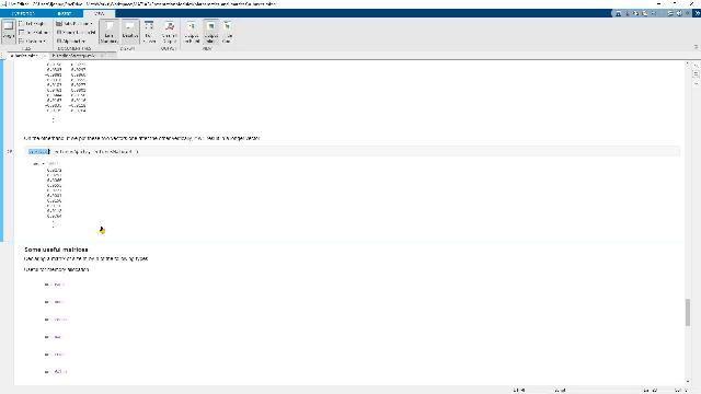
This brings us to some interesting matrices that you have by default in MATLAB like the rand matrix, ones, zeros. Let's go ahead and look at what this does. doc rand. So the documentation is a rich aspect of MATLAB. Just by looking at doc and rand, I can easily identify what this function does. So rand, it creates a uniformly distributed random numbers for the size that I specify. Let's go ahead and have a look at what that does.
So rand of one gives me one uniformly distributed random number. If I specify two, it gives me a two by two matrix of random numbers. If I want it to be of a specific dimension, such as two rows and five columns, then I specify the size, and then I get that. Using similar logic, I could ask for a matrix of ones, matrix of zeros, matrix of true values, false values. So these are logical arrays.
That brings us to the end of the first section where we were looking at how to work with matrices. Now let's go ahead and look at how to compute some simple statistics. So the first four moments of computing statistics, so mean, standard deviation, skewness, and kurtosis. So these are the functions for computing each of these moments. If I just go ahead and execute this, I get the mean of the returns matrix, standard deviations, skewness, and kurtosis.
Let's just go to the command window and have a look at what that gives. So that's my returns matrix. So that's exactly what I have here. If I compute the mean, I get two different numbers. First one is the mean of this column over here. And the second one is the mean of this column over here. So what I'm getting is the mean of returns of Apple and the mean of returns of Walmart.
Now what if I want the mean of returns of each of these stocks across each week? So let's say I want the mean of these two returns over here and the mean of these two returns over here, and these two returns over here. So for doing that, I could use the same function but not specify the dimension along which I want the mean to be calculated.
So mean on the second dimension. So instead of getting just two numbers, I get a column vector of numbers. So now I get much more values of mean. So that corresponds to the value of mean for these two numbers in the first row, mean of the value of these two values in the second row, so on and so forth.
Now that's with computing simple statistics. Now let's go ahead and start looking at element wise operations. So our strategy is a simple strategy. We are going to create a simple portfolio where we progressively buy increasing number of shares of Apple. Let's say in quarter one, we buy one share of Apple, in quarter two, we buy two shares of Apple, so on and so forth. And we'll see how we will create that quantity and how we look at the prices.
So let's extract the prices of Apple over here. So for doing that, it's simple. We go ahead and extract all the rows and all the values that we have in the column AAPL. Doing so, we get a subset of the prices of Apple that we pulled in from our Excel sheet. I can already observe that I have couple of missing values here for 5th January, then I've got the value on 8th January. It seems like I'm missing the values of weekends.
Now I'm going to complete this table. Why? Because I'm going to be observing the values that I have at the end of quarter, without worrying to have to look at if it is a working day or not. So let's say if I'm looking at the 31st of March, I don't want to worry about the fact if it is Saturday or Sunday or if there's a price for it. So if I just go ahead and complete this table by using the last available price, I should be able to just go ahead and pick up the last available date.
So for doing that, I'm going to be using a live task, which I have used from here, Task and Realtime Timetable. In doing so, I'm specifying that I'm looking to complete my timetable by every time step of one day and [? prove ?] that there's a missing value using the previously available values. Let me just go ahead and execute this.
So now you can see that I have more rows than before. So initially, I just had roughly 500 rows. Now I have 723 rows. So 4, 5 January, then I have 6 January, 7 January, and 8 January. So what has happened over here is using this live task, I've used the last available value, and I forward filled it until I get the next value. And you can see that this value have been updated for the entire table.
I'm storing the output of this operation into a variable called retainedPrices. So this is all the prices. Now if we're looking at the dates required, let's use this function called dateshift. So what that does is I'm looking for all the end of quarter values starting from beginning of 2018. So the format is so. So I start by specifying what's my beginning date. What am I looking for? I'm looking for ending values for each quarter, and I want seven of such units.
So I get 31st of March, 2018, 30 June, 2018, 30 September, 2018, so on. And I get seven of those values. If I had specified seven, I would get until 31st of December, 2019, but I know that my table does not go until 31st of December, that it stops at 27th of December. So I get quarter ending values until 30th of September, and then I add the last value manually, using the function that we saw earlier for horizontal concatenation.
So now thus far, we have identified what dates we require, and what column we are looking at. So this is the quarterly prices for Apple for end of each quarter. You see that we have no missing values. We are looking at four quarters for two years. So we are looking at eight values. Now the strategy that we identified was to look at progressively increasing number of shares every quarter. So if I use this command, which is to get a vector-- let's just go to MATLAB-- one to eight, I get a vector that goes from one to eight. So in quarter one, we have decided to buy one share, in quarter two, we have decided to buy two shares, until in quarter eight, we have decided to buy eight shares.
Now let's just go ahead and look at quarterly prices. quarterlyPrices.AAPL. So this is the prices of Apple that we have. And this is the numShares that we have identified. Now this price vector does not look like the number of shares. So for making the number of shares look like the price vector, we could take the transpose by using the single code right next to this variable.
So now you can see that the price vector and the number of shares look similar. Now what we're going to do is we want to multiply this price by this value over here for the first quarter, the price of the second quarter by the number of shares for the second quarter. So what we are looking at-- quarterlyPrices.AAPL multiplied by numShares. We are expecting a matrix of a similar dimension. Now we'll see what we get.
So MATLAB tells me that this is an error. That it has got incorrect dimension for matrix multiplication. So what that means is while using this operator, MATLAB is trying to perform a matrix multiplication of this vector and this vector. And for matrix multiplication to pass, it needs to have the inner dimensions that match. So for this operation to work-- so the dimension of this matrix is eight by one, and the dimension of this matrix is eight by one as well. And for our matrix multiplication, we want it to be of size-- this one has a size of eight by one, and this one has a size of one by eight.
So when we are performing matrix multiplication, the inner dimensions must match to get a matrix of the size of outer dimensions. If I just go ahead and do this operation, this should not result in an error. That list does not give me what I'm looking for.
So in order to get what I'm looking for, which is a vector of how much money I have invested in Apple, which I would get by multiplying the prices times the number of shares, I use the dot operator to multiply each element of prices with each element of number of shares. I'll just multiply that to that. So now I get something of the same dimension. But it does not look familiar.
So for visualizing that in a format that I'm more familiar with, I use the command format back. Now if I re-execute this command, I will be able to understand easily what the values are. So here's the prices for Apple. So the first value gets multiplied by 1. The second value, 180, gets multiplied by 2. The third value, 220, gets multiplied by 3. So on and so forth.
So we saw that. Now we have quarterly prices over here, and we see that it starts at 162. If we want to rebalance that, or if we want to rescale that to one, we go ahead and convert these prices into returns. And then reconvert these returns into prices by specifying the starting value that I'm looking for. So now the prices start at 100.
And that brings us to the end of the first demo. So we saw how we work with matrices. We looked at some interesting matrices. And we computed some simple statistics. We also explored how to perform element wise operations.
Now for the next demo, let's take a case study of doing a trading strategy using regressionLearner. And in this particular exercise, we'll be looking at how to fit distributions, how to identify trends using regression, and scaling up. Let's switch back to MATLAB. Let's go ahead close that as well. The script that I'll be using for that is the second script here, trading strategy.
So let's start clean. So clear. So the model is simple. So we start by importing the time series that we're looking at. We try to understand the statistics. We create some predictors for our model. Then we fit a model, make some predictions, and then we try to see what we can do from further up here. What are the possibilities that we have? And we'll close the session by looking at how to actually perform multiple tests using Regression Learner app.
So let's just go ahead and import the time series that we're interested in. In the first script, we looked at how we imported the entire price series. Now in the second script, we are not going to do all that. We are just going to import the price series that we're interested in. So here you can see by doing readTimetable, I'm just bringing in the prices of Apple from this Excel file.
And for doing that, I've used this function called detectImportOptions. If I look at opts, which is the variable into which I've stored the options, we can see that I have selected the variable names over here to import from that Excel file, which are specified over here, import opts.SelectedVariableNames is just that.
Now my strategy is to look five days into the future-- well, we're making a prediction for five days into the future. This number is arbitrarily chosen. It could be any number of days into the future. The closer you are, the smaller number of days you're predicting into the future, the more accurate you are. The further into future, the more unclear or less precise your prediction is. So I'm just sticking to five days, which is the number of working days in a week.
Now to ensure that my prediction falls on a weekday, I am looking at the simple test by looking at this function called weekday to ensure that I have no Saturday, Sunday in my data set. So I get two different outputs First output is dayNumber, second output is dayName. If I do a unique string of dayName, I see that there's no mention of Saturdays and Sundays in my data.
To compute returns, we use the function that we saw earlier, which is tick2ret. And then I use zscore, a function to standardize the returns that I've obtained. What does that mean? So to get an idea of that, I use a look at the documentation by pressing F1 or by right clicking and choosing Help on zscore. So what does that do is it removes the mean from each of the values in the vector, and it divides by standard deviation. In doing so, I'll have a mean of zero and standard deviation of one.
So let's go ahead and fit normal distribution on these returns. So in the first one, we see that the mu that has been fit has some value and the sigma as well. However, when I fit a normal distribution on my standardized returns, you can see that the value that has been observed for mu is zero. And the one for sigma is equal to one.
Now you can do this distribution fitting visually as well. So for that, you have this app called Distribution Fitter, which you can access by this command, or you could go to the Apps Gallery and find Distribution Fitter, which is an app. It is the same app that we access by using command line. So that's what that looks like.
Let's go ahead and import data. No data sets have been created. standardizedReturns. Create Data Set. Close. Now to create a fit, I go ahead and choose New Fit. And let's say I'm fitting normal distribution. Apply. And you can see it fits a normal distribution. I can play around with other distributions over here. So logistic regression, lets say Apply. And you can see how this one fits the data.
So you could use the app to further fit more distributions or fit your data closely with another distribution. Now in the second bit, we are looking at these statistics. So we saw how to compute statistics previously. In the next step, we are creating some technical indicators for creating our regression problem.
So we know the response variable is the prices five days into the future. Now for arriving at that, we need to have some predictors. So we're going to create them using technical indicators. So here, I am using a five day moving average and a 20 day moving average. What that does is that it smooths out the prices and using a simple rule of crossover, which we wouldn't bother to write the rules for. We would just let MATLAB figure it out.
We are going to create some predictors to feed into our regressionLearner problem. So here's an example of two of these predictors. In the next step, I'm using a lot more of this. So if I look at the function name, if I click on it, I see that there's a blue bar over here. And that corresponds to line number 27. There's a second line over here, which seems to be the declaration. So if I click on it, takes me to that second line. And I can see that's the same function. And it's computing all these technical indicators within this function. And it returns that and this variable here. To go back, I click on that, I click on this bar over here, and it takes me back to where I was.
On execution, that's what I get. Here's the beginning portion of a technical indicators table. And this is the ending portion of the table. Now for creating a response variable, we are looking at five days into the future. For doing that, let me put these two together. So this is the Apple table that we have, and this is the future value. So I'm taking the fifth value from here and placing it over here, the sixth one over here, the seventh one over here.
Now what I'm going to do is I'm going to take this table and merge it along with this table over here, technical indicators. And I remove missing values and thereby creating a clean value of my table over here. So thus far, I've got my data. And we're going to fit a linear regression model onto this data. So for doing so, I've got this function fitln, and this is my data, regressionData.
Just go ahead and execute that function. And here, you can see the equation that has been fit on this data. This last variable in the table has been identified as the response variable. And this is the equation that has been fit onto our model. This is the model object. I can open this in MATLAB using Open, Control-D. Or open mdl_lm. And here, you can already observe what are the residuals of the linear regression, the data itself that we sent into the model, the coefficients of the model.
Here, I can observe the r-squared of my model, the error of my model. We can see that there's a lot of information that comes along with this model object. To have a look at other possibilities with the model, I look at the methods that have been defined for the model using methods of this object. And you can see that there are couple of plots that are associated with this model object. Let's just go ahead and look at plot, mdl_lm, in which case, I can see the line that has been fit onto our model.
So this is exactly what we just saw, plot(mdl_lm). For more information and for other kinds of linear regression, I encourage you to go ahead and look at the documentation by typing in this or by executing this using F9, in which case, you can see the other possible linear regressions that you can perform. Let's say generalizing your regression, Bayesian regression, and so on. You have 693 pages to explore.
To make predictions using this model, I use this function called predict. Specify the model, and then if I have a test set or a validation set, I could specify that here. And then I get the predictions. So this is the predicted values from the model. Here, I've made a plot of what the actual values are in the test data against the predicted values.
Now thus far, we saw how we import data, how we create certain problem for regression analysis, how we actually work with models, how we fit a linear regression. Where do you go from here? There are a couple of directions that you could take with your project. One is you could think about dimensionality reduction. The next aspect is you could think about splitting a data set into two, which is a training set and a test set. You could even think about productionizing your code, writing professional-level code.
Now Regression Learner, we will see in a minute, is one way to do all those things together. So let's create our data set by splitting the regression data into two. So here, we are going to split this into training set and test set, dataTestRegressionLearner and dataTrainRegressionLearner. We're going to split it into a 60-40 split. So there'll be 60% of you data in training set, and 40% of your data in test set.
And for working through the app, we use the Regression Learner app, we execute this code here. It opens the Regression Learner app. I import the variable from Workspace. I choose dataTrainRegressionLearner. It has correctly identified the response. If this is not the correct one, you could choose what is the correct response here. These are all your predictors. The default validation approach is cross validation. Let's leave it at that. Start Session.
Now here, I have the possibility to choose all the models that I have at my disposal over here. I can also [? think ?] of dimensionality reduction using the PCA technique. I could employ parallel computation. So let's just go ahead and choose All Quick To Train Models. And then click on Train. Now this is searching on the parallel pool, which I will leverage to train multiple models in parallel.
So now that I've got the parallel pool open, let's go here and click on Train. So you can see that it's training four models simultaneously. And the error associated with each of these models is displayed with each of these models. Let's say this is the model with the least error. If I change the model, you can see how the model fits the data. So looking at the model with the least error, we see that there's a reasonably good fit.
This is the response block. To look at how the predicted values fit with the actual values, you can look at that. The residuals plot. You can also have a look-- you can also export this figure or create a function for this model. What we are going to do is export this model into our workspace as a trained model. So let's say ourTrainedModel. So into this variable, we save this model that we just created.
OurTrainedModel. So it tells me how to predict it by looking at this field. It tells me I could use the predict function. So ourTrainedModel. predictFun(dataT estRegressionLearner). And here, it makes the prediction for the new data.
And with that, we come to the end of the second demo. So in the second part, we saw how to use the distributionFitter app, we identified trends using regression, we scaled multiple models, we scaled our data to fit onto multiple models, we used parallel computing, and we created production-level code using Regression Learner app. With that, we come to the end of our session. Thank you.
Featured Product
MATLAB


Select a Web Site
Choose a web site to get translated content where available and see local events and offers. Based on your location, we recommend that you select: United States.
You can also select a web site from the following list
Americas
- América Latina (Español)
- Canada (English)
- United States (English)
Europe
- Belgium (English)
- Denmark (English)
- Deutschland (Deutsch)
- España (Español)
- Finland (English)
- France (Français)
- Ireland (English)
- Italia (Italiano)
- Luxembourg (English)
- Netherlands (English)
- Norway (English)
- Österreich (Deutsch)
- Portugal (English)
- Sweden (English)
- Switzerland
- United Kingdom (English)