MATLAB Reservoir Simulation Toolbox in Action

Hi, my name's Francesca Watson and I work at SINTEF Digital in Oslo. And in this presentation, I'm going to show you some examples of using the MATLAB Reservoir Simulation Tool Box, or MRST for short. If you want more information about MRST, you can have a look at the talk by Knut-Andreas Lie, which talks about using MRST for carrying out reservoir simulation in MATLAB.

So in this presentation, I'm going to be going through two examples. In the first example, we're going to build a model from scratch in MRST, and we're going to run the simulation model. And in the second example, we're going to import a model from Eclipse, run the model in MRST, and then have a look at some simulation post-processing using flow diagnostics.

So first of all, to get hold of the software you need to go to our website, which is mrst.no. And then you can download the software which comes as a zip file. To install it, you need to unzip that file, navigate to the folder where it's stored, and run the startup script. Running the startup script will set up some of the paths that you need to use to load all the necessary modules for your simulation.

It also gives you, as you can see in the command window, a list of helpful hints. And one of the main things that you need to look at when you first get into MRST are the examples. So if you type in MRST examples, you'll get a list of all the examples from the core module. And all the modules have examples in them, which have some very useful functionality for setting up different types of problems.

So the easiest way to start using MRST for yourself is to find an example which is closest to the thing you want to do and then modify it. It's also possible to find examples for different modules. But for instance, if we wanted some examples that used the black oil modules, then we could type in MRST example, ad-blackoil. And that would give us a list of all the examples for the blackoil module. So that's a good way to get started.

So in this first example, what I'm going to go through is how to set up a simulation from scratch. If you already have an eclipse deck, then you don't need to go through all these steps. You could just load the eclipse module in and run that simulation in MRST. But I'm going to show you how to set up something from scratch.

In the editor window you can see the example script. And all the examples that we have for the different modules have examples that are set out in a similar way. So the idea is that you can run the example cell-by-cell, and there's some handy information saying what's going on in each cell to help you figure out how to use the software and see what it's doing.

So as I said, this example, we're going to build and run a two phase blackoil simulation from scratch in MRST. Now the first thing we need to do in the first cell is add some modules. So here we're using the ad core module. So ad stands for automatic differentiation.

And here we need to input the ad-core module, which has the simulated framework, the ad-blackoil module because we're running a blackoil simulation, ad-props module which has some functionality for setting up fluid properties, and the mrst-gui module which has some plucking functionality. So if I run this cell, you can see in the command window you now have a list of the modules that we have currently loaded in MRST.

The next thing you want to do is start building our grid. So the way we're going to do this is by building some horizons and then converting those horizons into a grid. So this cell sets up a single horizon just in MATLAB. So if I run the cell, you can see it plotted in the figure window. And we have a simple horizon that's set up using some x y zed coordinates.

In the next cell, we want to add a couple more horizons. So yeah, we'll run the cell and you can see there's three horizons now. The green horizon and the red horizon and then the blue horizon actually has an [? erosional ?] surface, so we're going to model a print out between the blue and the green. So now we have these horizons set up, we can move on to the next cell, which is going to convert them into a grid.

So the first function that we need is this convertHorizonsToGrid function, which will create a cornerpoint grid by taking the services and extruding them out and making grid cells. And then we're going to use processGRDCL to create the MRST grid structure, which is a capital G. I will run this now and you can see in the figure window that the black lines are the outlines of our grid.

In the next cell, we would like to put some faults in. So this is to demonstrate how easy it is to modify the grid in MRST. In order to put some faults in, what we've done here is we've modified some of the zed-coordinates. And then we've reprocessed the grid and computed it again. So I've run that cell now.

And you can see on the right hand side, a grid with some faults in it. And this is colored just by layer number so you can see the different layers of cells in the model. So now we have the grid setup. We need to add some petrophysical properties. So this needs the porosity and the permeability for the grid cells.

So the permeability that you want to use are like normal permeability distribution in four different layers. So I will run this cell. And you can see in the image that we have different permeabilities throughout the model. We've also set up a porosity value of 0.3 for all the cells in the model. And then we use makeRock function to generate a rock structure in MATLAB, which has two fields, one poro and one perm field.

Moving on to the next cell in the script, we need to add some wells. So in this model, we're going to have three production wells, which are controlled by a bottom hole pressure and one injection well, which is controlled by injection rate. I won't go into details of how to set these up. But if you have a look at the help file for the vertical well function, it will tell you what all the inputs are.

If I run this though, you can see plotted on the grid are our four wells. Three production wells, and one injection well. Moving on, now we need to set up a fluid. They do this using the function initsimpleADIfluid. And in this case, we're going to have two phases. We're going to have a water phase and an oil phase.

We set the viscosity for both phases, the density for both phases, and we've also got this end parameter, which is the exponent where the rel perm curves. It should be the same for both phases. If I run this cell, you can see plotted in the command window the fluid structure.

And the thing to notice about the fluid structure is that quite a lot of the properties, such as the rel perms and the viscosity are actually set using anonymous functions. This makes it very easy to move functions in and out and replace them. So in this case, you set constant water expansion at water be effected. But the b effect of the oil, we have changed the function for that so that we can have some compressability in the oil phase.

Moving on to the next cell in our script. So now we have the grids and we have the rock and we have the fluid. But we need to set up the model which will set up all the equations for us. So we're using a two phase oil water model here. And if I run this cell, I set up the model. And also we can use the function inspectFluidModel to have a look at some of the fluid properties that we just set up in the previous cell.

So here I'm plotting the densities. You can see that we have constant water density but increasing oil density with pressure. And it's also possible to look at different properties using the list on the right hand side.

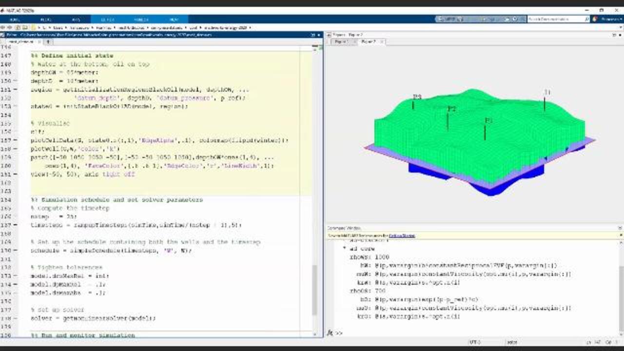
Next, we need to define an initial state for our reservoir. So the way we've done this is we've set the oil water contact at 85 meters. And then we've run this cell and we will get a-- and in the figure, you can see that we have oil above this oil water contact, and water below the oil water contact, which is shown by the gray plain.

So finally, we need to set the schedule and we need to set up the solvers. To set up the schedule, we create a list of time steps. And then we use the function simpleSchedule where we pass in the time steps that we just created and also the well structure that we created earlier on. And that will create the schedule for us.

And then to get the correct solver, we use the function getNonLinearSolver with the model that we made. And this will look at the model and look at different properties of it and choose the most efficient solver to use in this case. Run that cell. And then finally we can simulate our model.

So the function for simulating is simulateScheduleAD. We pass in the initial state, the model, the schedule, and the solvers that we've just generated. I've also given it a function called afterStep function, which will allow us to do some plotting as we're going along through the simulation.

Then I have set this running. You can see in the bottom right hand corner, we have some output to the command window about which time step we're on. And we've also plotted some figures.

So the figure that you can currently see has two progress bars. The top progress bar shows you the percentage of control steps which we've gone through. And the one underneath it shows the simulation time which has passed during the simulation so far. We also have a plot underneath that, which shows the number of iterations per each control step.

We also get some print out here where we have a plot of the water saturation as it's progressing throughout the simulation. And you can see how it changes after each time step. And then finally, in the third figure we are plotting some of the well solutions.

So in this figure, we have plots for the three production wells, and we're plotting the water cut. And you can see that as the simulation progresses, the water cut is increasing for the different producers that we're having. You can also have a look at the different menus. So we don't just have to plot the water cut, we can also, if we wanted to, plot the reservoir rates for the water or the oil or the total rates and the surface rates and we could plot the bottom hole pressures.

You can change the unit system, and we can also change the axis of the grid that we're plotting on. So now if we look at the bottom of our command window, you can see that the simulation is complete. So we have all our results. And if we go back to this window, then we could have a look at some of the other things as well as the saturation.

So this is just the pressure at the final time step. We can have a look, for instance, at the pressure at the first time step. Or if we wanted to watch how the water saturation changed throughout the simulation, we could select the water saturation and then play this and have a look at how things change throughout the simulation.

So that was the end of the first example. And now we'll move on to the second example.

So in this second example, I'm going to show you how to load a model that we already have as an eclipse deck, import it into MRST, and run the simulation in MRST. And then we're going to look at some low diagnostics and post-process the results that we have.

So all the things that we did in the first example-- so setting up the grid and the schedule and the initial state-- if we already have an eclipse deck, then we don't need to do that. You can just import that directly.

So to begin, we need to add some modules again. We need to have ad-core and ad-blackoil. And we also need the deckFormat module because this has the functionality for inputting the eclipse deck. Now you can see we have these three modules that are active at the minute.

Moving on to the next cell. This is where we can read in and set up a model. So the model that we're going to read in is a brugge model. And we can use the readEclipseDeck function to read that in. And then we can also use initEclipseProblem ad which will take that deck and will set up all the things that we did in the previous example.

So this will give us the initial state, the model, the schedule, and the solvers. I've run that cell. And you can see it's finished now. And in the window, you can see a plot of the oil saturation for the model. You can see that actually the initial saturation in this case is non-uniform. So we have oil in one part of the reservoir and water in the other part.

The next cell in the script, we'll set up a packed simulation problem. So this is slightly different to how we did it earlier. But using the pack simulation program, we can collect together all the things that we need to run a simulation-- so the state and the model and the schedule-- and then we can collect it into a problem structure and we can simulate the model using simulatePackedProblem.

So the advantage of doing this is that this simulatePackedProblem will save the simulation as it's going on. So it allows you to load a simulation that has already been run. But when I run that cell, you can see that actually I already ran the simulation earlier, so we don't need to rerun it again here.

If you want to get output from the packed simulator problem, you can use the function getPackedSimulatorOutput here. So I run here and that will load everything that you would get from the simulation into the workspace so you can inspect the results. But actually in this case, what we're going to do here is do some flow diagnostics.

So move on to the next cell. And here, to run the flow diagnostics, we need to add a couple more modules. So we need the mrst-gui module, some plotting output, and we need the diagnostics module to actually do the flow diagnostics. Then we run the function PostProcessDiagnosticsMRST.

We'll set the cell running. And what this is doing is it's computing some flow diagnostics for our simulation results. So flow diagnostics are just some simple quantities that we can calculate based on the flow field. And they allow us to inspect how the flow fields are connected visually in a 3D sense throughout our model and look at different regions in the model in which wells are connected to each other.

So now we have these plotted, we can see in the viewer here that we have loaded some time steps on the left hand side. And we also have, in the main window, a picture of the model grid. And the model grid is showing the porosity at the minute.

So you can see in this window-- if I move this around, we can inspect our model and have a look. If we want to look at some different properties, we can have a look at the permeability perhaps. And if I plot that and then I click the log10 button, then you can see the permeability a bit better.

Now I'm going to select a time step here, and then I'm going to have a look at where the wells are. If I select auto detect well pairs. And then I'm going to select all of the injectors. And the auto detect well pairs knows that all the injectors are in fact connected to all these producers, so I can plug all the wells. So you can see in this picture here, we have the injector wells in blue and the production wells in red.

Next, I think I would like to look at some flow diagnostics for this model. If we look at the flow diagnostics, I will go to this menu here and click on Diagnostics. And then I think I want to look at some sweep regions. So the sweep regions are just the regions that are swept by fluid from a particular injector within the model.

But this time so that we can see we have four different sweep regions. And if I scroll through the time steps, you can see how these sweep regions change. And you can also notice that we're getting more and more colors visible. So in order to find out what's going on, I'll have a look at the simulation output here.

So for the stimulation output, what I'm going to do is I'm going to select all the injection wells and then I'm going to plot the water rates. You can see in this plot on the bottom left that actually as you move through the simulation, the wells are being turned on through time. So consecutively, different wells are coming on at different times, which indicates why we're getting more and more sweet regions showing up in our sweet region plot.

Another thing that we can do is look at the well allocations. So if I go to the well allocations menu here, then what I want to look at here is the well connection matrix. So this matrix shows how strong the connections are between the different wells. If you have a yellow color, then there's quite a strong connection between those two wells because quite a lot of fluids are flowing from between those two wells.

So in this case, we have if we look at injector 10 on the second line here, we can see that has quite a strong connection with producer 11, but quite a weak connection with producer one. And if the cell is white, then there's no connection at all, in this case. So now we've looked at that. I think I want to have a look closer at one region.

So I'm going to pick the region around injector 6 and then I'm going to threshold this region so I can only see the flow paths that are involved in injector six at this time step. But actually, I would like to select all the time steps and have a look at what's going on throughout the whole simulation. And what I would like to plot is the oil saturation.

So I'll go down to the dynamic selection here in this property display box and S oil is the oil saturation. But I also like to get a bit of a closer look. I can turn the grid off here and that will zoom into this region. So here we can see that we have the oil at the top in yellow and water at the bottom in blue. And we also have two different sets of producers.

So the producers on the left hand side are directly connected to injector six. And then there's a water lag all the way down at the bottom. And then there's a group of producers on the right hand side, which also appear to be connected. So this indicates that there is some pressure support from injector six all the way to this group of producers on the right hand side.

But what I'd be interested to know is, is the fluid that is being injected at injector six actually traveling all that way and going into those producers. So to do that, I'm going to have a look at some more flow diagnostics. In this case, I'm looking at the time of flight, forward time of flight.

And the time of flight is the time taken for a particle to travel from an injector to a particular point in the middle. So in this image, you can see the blue regions have quite fast time of flights. But the yellow regions have a time of flight of around about 500 years. So actually this suggests that the fluids are not traveling all the way down towards the second group of producers. But there is some pressure support between the injector 6 and that group that producers.

Another thing we can look at if we want to look at how the fluids from injector six are flowing is we can look at the allocations. So I'm going to select the final time step here, and then I'm going to have a look at the injector allocations. So in this plot, you can see what percentage of the flux from injector six goes to which producer.

So basically, here we can see that most of the flux from injector six is going to producer four and producer 16. Another thing that we can look at are the actual profiles. So on the right hand side, you can see the injector profile, which shows the cumulative allocation from the toe, which is down here, to the heel of the well. And this shows you how much of the flux is traveling to each different projector from each point in the well.

So that was a very quick introduction to some of the functionality you have in MRST. We have a lot more functionality and a lot more modules that do various different things. We also have a lot more functionality within this flow diagnostics gui, which I haven't had time to show you. But if you'd like to check out our website, you can find a lot more information there. Thank you very much for listening.