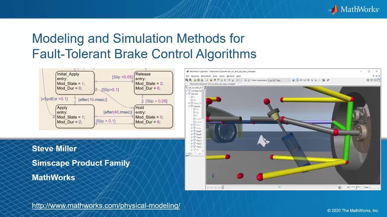
Modeling and Simulation Methods for Fault-Tolerant Brake Control Algorithms

Hello. My name is Steve Miller. In this presentation we're going to learn about modeling and simulation methods for developing fault tolerant brake control algorithms.

To see the effect of component failure on an anti-lock braking system we have two models of a vehicle. In one vehicle, all components are operating properly. In the second vehicle, one of the valves is going to fail. This animation shows the simulation results for both vehicles.

The vehicle with the failed component has a longer braking distance and the driver has a more difficult time controlling the vehicle. If we view the same results from within the vehicle and look at the wheels, we can see the effect of the failed component.

The blue vehicle with no failed components, the wheels do not lock. But in the orange vehicle the wheels have locked, leading to a longer braking distance and poorer steering performance. In this presentation, we'll see how to create this model so we can develop an algorithm that tolerates this failure more gracefully.

Here are the key takeaways for this presentation. We will see that simulation enables engineers to detect the impact of degraded components on overall system performance. We can model failed components, such as valves that stick open or stick closed, in order to assess the effect of failure on system level performance.

Next, virtual tests that integrate control software and failed components make it possible to develop fault tolerant algorithms. By integrating these components with a model of the control algorithm we can see how it handles these failures and then develop algorithms that handle them even better.

And finally, developing fault tolerance algorithms requires automating tasks and methods to accelerate simulations. In a vehicle there are many combinations of faults that can occur at different severity levels. We will use MATLAB scripting to automate those tests and parallel computing to accelerate the running of all of those tests.

Here's the agenda for our presentation. We have seen the effect of component failure on an anti-lock braking system. We will see how to develop that model as a digital twin including hydraulic, mechanical, and electrical systems, as well as the control system. We will then look at two categories of faults and an anti-lock braking system-- modulator failure and sensor failure. And then we will assess the effects of those failure on system level performance.

Here is the workflow we will go through. We'll model the vehicle, the control algorithm, add faults, and assess the impact. That will allow us to refine the algorithm to handle those faults more gracefully. The purpose of an anti-lock braking system is to help drivers retain steering control by preventing the wheels from locking up during an episode of heavy braking. Skidding tires provide less traction, which means longer braking distance, and poorer steering performance.

To prevent locking the sensors detect wheel speed. The software will then determine if the wheel is skidding. And the software will control the brake pressure in order to make sure the wheel does not skid. In a car, sensors measure how fast the wheels spin. When the driver applies pressure to the brake pedal, that pressure slows down the wheel.

The control algorithm detects that the wheel has stopped and knows that it is skidding. It can control the amount of pressure applied to the pedal through a set of hydraulic valves. The control system will then release pressure to the wheel so that it will start spending again. Once it is spinning fast enough, the control system will adjust the valves again to slow the wheel down.

By cycling this pressure, the control algorithm can search for the point where the wheel has maximum traction. Here you can see this in an animation. The red cylinders indicate the pressure at the wheel. You can see that when the pressure increases the wheel speed slows down. And then when the pressure is released, the wheel speeds up again.

To model this system we need a model of the vehicle, the hydraulics, and the control algorithm. Here you can see some of the simulation results. The brake pressure is cycling up and down and the wheel speed is cycling up and down as well. If we zoom in on a portion of these results, we can see that the brake pressure goes up in steps and the wheel speed goes up and down.

The wheels spin at a varying speed in order to maximize traction. The control system is hunting for the amount of pressure that will lead to the wheels having the maximum amount of traction so we can get better braking and steering performance.

Here is an overview of the vehicle model that we are using as a digital twin. The model includes a mechanical system, hydraulic system, sensors, and the control system. A multi-body model makes up the suspension and the chassis. A hydraulic network is used for the braking system, including the master cylinder, the caliper, and the valves that control pressure at the wheels. And the control system is modeled as a state chart.

To run this test we need more information. We also need information about the environment or a model of the road surface, model of the driver, and measurements that are sent to the control algorithm. The mechanical model of the suspension looks like this. If we look at one corner we can see that we have modeled a double wishbone suspension and the steering linkage.

We have combined generic 3D geometry for the linkages with the CAD model of the braking system. By combining these two elements we have realistic geometry, as well as parameterize components so that we can adjust the design.

The braking system is modeled as a hydraulic network. This is referred to as a 4 channel 4 sensor system. We have a tandem master cylinder, brake lines. This portion of the hydraulic network represents the front left channel. It has one valve so the control system can increase pressure to the brakes, and a second valve so that the control system can reduce pressure to the brakes.

The control system can take three actions. It can apply or increase pressure at the wheel, it can hold pressure at the wheel, or release pressure from the brake caliper. It can do that by adjusting the two valves I showed you before. The decision as to whether increase, hold, or release pressure is made based on wheel slip.

Wheel slip is an estimate of how much the wheel is skidding on the ground. This is estimated using sensors, both wheel speed and accelerometer. The sensor data for all four wheels is sent to an algorithm to estimate the vehicle's speed and the amount of wheel slip. This information is then fed to another part of the algorithm which decides whether to open or close the valves to adjust the pressure.

Here you can see a very basic anti-lock braking system algorithm that has the states I described-- apply, hold, and release. We'll go through one of the cycles so you can see how the system works. In the wheel slip plot you will see how much the wheel is slipping. A high amount of slip means the wheel is skidding. Low slip means the wheel is rolling along the ground.

And in the second plot you can see the valve commands, the signals to the apply and release valves. At the start of this test the braking system is inactive. The driver has not stepped on the pedal. When the driver steps on the pedal the brake pressure increases, as shown by this cylinder.

Once this red cylinder extends too far, you can see that the wheel slip has increased. The braking system must release pressure. So it adjusts the valves to reduce pressure at the wheel. The wheel will then start to accelerate and the wheel slip will go down. Once it gets below a certain threshold, the control system will then reapply pressure to the system. It adjusts the valve commands to increase pressure at the wheel.

We can see that it is increasing in steps. Once it reaches the target level of slip the control system will hold pressure at the wheel. And once the slip increases to a higher level, it will again release pressure at the wheel. Going through this cycle, the control algorithm is searching for the condition where the wheel has maximum traction. It doesn't know what surface it's on. It only can tell how much the wheel is slipping based on its estimate. So it needs to cycle the pressure to find that level.

Now that we have our system functioning properly with the control system and the physical system, we will now model component failure. A common failure mode from modulators is valve failure. The valve can remain stuck open. It can remain stuck closed. Or it can have partial failure, where it cannot completely open or completely closed. This can affect the apply, release, or both valves.

You can begin to see how many combinations of failures and severity levels that can appear in the vehicle. Here is our model of the valve. And we have enhanced one of the standard valve models to include a fault mechanism. We can configure it to stay stuck open, stuck closed, or to permit it to only partially open or only partially close.

Here you can see the effect of this failed valve on one wheel where the valve remains stuck open and the wheel locks. So as long as the pressure is on there, because the control system cannot reduce pressure at the wheel.

Now we're going to run a test where we have a fault on the rear left apply valve. It is only permitted to close 50%. That means that the control algorithm cannot reduce pressure at the wheel and it will lock the rear left wheel. Here when we run our test we can see that the pressure on the rear left wheel is remaining on. The wheel is locked, which drastically prevents us from slowing the vehicle down and affects steering performance.

Here on this plot, you can see the comparison of the faulted behavior and the no fault behavior. And you can see the vehicle skids for a much longer distance. We can also see in the pressure plot the wheel-- the pressure at the rear left wheel does not go down to zero. And correspondingly, the wheel speed for the rear left wheel does go all the way to zero. That wheel is locked for the duration of this test.

This shows us that our algorithm is sensitive to valves failing. It cannot handle that condition gracefully. We would need to enhance the algorithm in order to make it fault tolerant.

Another common failure in anti-lock braking systems is sensor failure. The wheel speed sensor consists of a toothed wheel that's attached to the axle. It generates pulses that are fed to an electrical circuit which will generate a square wave for an active sensor or a sine wave for a passive sensor. And then this is decoded to figure out the speed.

Now, there are many ways that this can fail. Mechanical sources of failure include worn teeth, it can slip from the mount, low tire pressure will also cause a failure because it is assuming a radius. And if that tire has low pressure it will affect the radius. And there are also electrical problems that can happen with the effects of temperature or electrical noise in the system.

We can use simulation to measure the impact of failure on the signal that is used by the anti-lock braking system and then mimic that effect in the vehicle model. Here we have a portion of a Simscape model that represents the wheel speed sensor. We can introduce a fault in the decoding algorithm that shows that a tooth is missing.

So here you can see these pulses of low speed. We're mimicking the effect of a tooth missing on the wheel. For our test here, we're going to remove two teeth on the rear left wheel. This will cause longer spikes of low speed.

Here in this animation, we can see the effect of this fault. The pressure at all four wheels is cycling, including the rear left wheel. If we compare the plot of the path of the vehicle with the no faulted behavior, we can see that the final position is not too different and the steering is a little bit affected, but it's not too bad.

If we look at the wheel speed and the pressure signals we can see that oscillation has occurred. So this fault was not as severe for the system as the stuck valve. If we look at the measured signal we can see that the algorithm was fed the speed of the wheel speed signal that had these spikes of lower speed, but it was not particularly sensitive to that fault.

This is also a useful result. It means that this would be a lower priority fault for us to improve the algorithm and make more tolerant. We really should focus on our time on detecting the cases where there are faults in the valves. To assess the effects of failure we need to run many simulations. There are vast set of cases to test. There are many different types of faults, different severity of the faults, and locations of the faults in the system.

Even beyond the types of faults we're going to look at there are a wide range of road conditions, maneuvers, driver types, and so on. With all of these tests to run, it's critical that we shorten the time required to perform these tests. The key methods we use to shorten the time required to perform these tests include automating the configuration of the model using scripts. We can start the simulation at the event and use parallel computing.

To run these tests, for us, the most interesting part of the simulation is when the vehicle is at speed. So to shorten the time it takes to run these tests will run the portion of the simulation where we get the vehicle up to speed. We run that once. Save that operating point and run all the tests starting from there.

You can see that we can save more than half the time by running from this operating point. Ideally we wouldn't run them on just one computer. We would distribute the simulations to multiple cores on a single system or across a computing cluster. This will allow us to shorten the time it takes to sweep through all these fault conditions.

Here are the keys to leveraging this approach. You need to have a model of the physical system and the controller with the relevant physics. You need to capture the behavior of the entire system. So you need to have the control algorithm, the hydraulics, the mechanical system, all in one model. But you need only enough detail to capture the effect of the fault. But you don't want to capture so much detail that the simulation becomes very, very long.

It's important to have a good understanding of the mechanism of failure and the effect on the system. Not to put in too much detail that doesn't really give you any additional help. Because of this, it's important to have access to multiple modeling methods. And abstract expression of a fault can be the most useful one.

If you understand the impact on the system, you can create a model that gives you what you want and runs quickly. If you do have access to models that are very, very detailed, you can get simulation results from that model and tune your abstract model to match that behavior. In this way, you have an accurate model that runs quickly.

Here are the key takeaways from this presentation. Simulation enables engineers to detect the impact of degraded components on overall system performance. Virtual tests that integrate control software and failed components make it possible to develop fault tolerant algorithms. And finally, developing fault tolerant algorithms requires automating tasks and methods to accelerate simulations. Thank you.