Nonlinear Confidence Bands Computation in MATLAB
Kadir Tanyeri, IMF
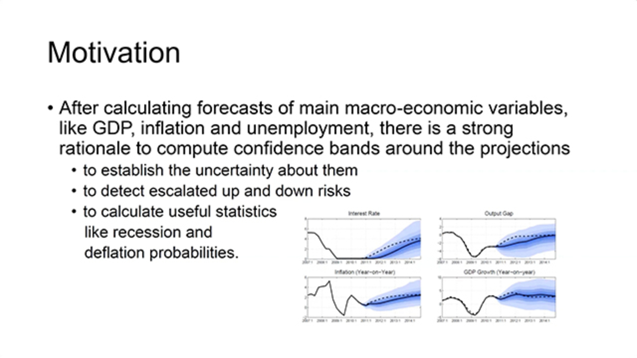
The global dynamic stochastic general equilibrium model for forecasting main macroeconomic variables like GDP, inflation, and unemployment is nonlinear. There is a crucial need to compute confidence bands around the projections in order to establish the uncertainty about them, detect escalated up/down risks, and calculate useful statistics like recession and deflation probabilities.
Confidence intervals are calculated by drawing samples from the estimated distributions of exogenous shock terms and each time solving the system of equations using a nonlinear solver in MATLAB®. The standard method, Monte Carlo sampling, is not practical due to the enormous number of drawings needed. We opted for a more structured way of drawing the shocks in order to more evenly sweep the high dimensional space—Latin hypercube sampling–which we have implemented in MATLAB. This sampling technique implies a faster convergence; in other words, a smaller number of simulations is needed to obtain good estimates of the confidence bands.
Furthermore, we do use distributed computing in MATLAB over a cluster of servers to speed up the process even further. System solution and calculations are sent to more than 100 workers on a cluster of several servers, then results are collected and compiled, which enables the whole calculation to be completed overnight instead of taking months if none of these methods were involved.
Published: 7 Nov 2023
Hi, everybody. I'm Kadir Tanyeri from Information Technology Department of IMF. Before starting, one of my older students texted me saying that he has seen these information on MathWorks site. He said my abstract was so complicated.
So I'm going to try to make it as simple as possible. So this is about calculating confidence bands using MATLAB, mainly. When we calculate forecast of a main macroeconomic variables, like GDP, inflation and unemployment, there is a strong need to compute confidence bands around the projections.
One of the main reason is to establish the uncertainty about them. We can say the inflation is going to be about 3% next year. But if we say it is-- we are 95% sure it's going to be between 0 and 10, that doesn't give much information.
It is much better if we can say we are 95% sure it's going to be between 2 and 4. So uncertainty comes from different sources, obviously. Modeling itself, the model itself. We try to make this as little as possible. Data is another source. That, we have less control, obviously.
But basically, we have to be able to communicate how sure we are about the forecast projections we are making. There are some other reasons. The model itself is a nonlinear model that comes from different reasons. It's a structural model, DSG models. And we use-- on top of MATLAB, we use modeling tools like Dynare, as Sebastian has presented a while ago.
So this nonlinear model can tell us actually if we can calculate confidence bands, if there are up risk and down risk. Today, we have seen the latest data on inflation. And currently, there is more down risk on the forecasted inflation than up. It is very important to be able to see that, say that.
More than that, we can also calculate useful statistics with this information like recession probabilities, deflation probabilities. Today, it is very important to say what is the probability that the inflation will be less than 4% in the next year in this country, another country, wherever, everywhere. So for all these reasons, it is very important to come up with confidence bands, calculate confidence bands around the projections.
So what do we require to be able to do that? First of all, we start with a suitable nonlinear macroeconomic model. We basically use a nonlinear dynamic stochastic general equilibrium model that Sebastian has mentioned, Dynare can deal with. The model is developed. It encapsulates most of the GDP of the world. It is fine. It is tuned frequently, and so on, and calculates at the end, a forecast about the macroeconomic variables.
Once we come up with this model, then we need a platform to solve the model efficiently. MATLAB offers whatever Toolbox we use on top of it, MATLAB offers great combination of tools for estimation. Estimating the parameters in the model, filtering, forecasting and running simulations. Its solvers and many others are very up to date, very efficient. They are running fine and fast. And we have verified that its solutions are as good as it gets.
We also need data on observable variables. Finding data is not that difficult, but we basically need to grab all the data on the fly when we are running the models. The latest data [INAUDIBLE] MATLAB has great functions to fetch data from multiple outside sources and clean it, transform it, and so on. Very efficient panel data functionalities. But our main point in this presentation is we need to run big number of simulations over the baseline because, as we said, the model itself is non-linear.
We have to run simulations. And then the number is-- we have estimated it is very large actually to make it converge over the long-term. To be able to run all these simulations in a workable time, we need a strong computer power, but also good combination of software with the hardware. We will-- we're going to mention about it in a minute-- we're going to need some help from multiple directions to be able to end up with a good time actually on the computation.
So model setup, I'm not going to go too deep in this. But basically, we have designed then implemented the model to cover all relevant macroeconomic dynamics in a modeling platform that is most suitable for the methods to be used. Basically, we use a Toolbox like Dynare, which runs on top of MATLAB and uses MATLAB's abilities. Here, I gave just one equation, but this model is full of equations like this.
And no matter what you do, it's a model, it's going to be missing something. But you want to include as much as possible to deal with current situations. So over time, we do change the models based on what is changing in the world and economics to be practical.
Data is very important. Whatever observables, we need all the data related with that in time, just in time. It is all collected and cleaned up and transformations all done in the code, on the fly. Just before we are running it, it's collected and used, basically.
And then the model needs to be solved. The model solution includes estimation of the model parameters. In General data in economic models are scarce, it is not that big. So we need to include expert opinions in terms of prior information in the models.
Then we have some of the variables observables. We have data for them. Some of them are non-observables. Whenever we have available as data would be noisy. We need to filter them to be able to get the noise out of it and also come up with series for non-observables.
And using all these after we can estimate the model and clean up and fix the data, we can run forecast based on forecast. These are all done in the modeling Toolbox on top of Dynare. So our problem starts after this actually.
To be able to run confidence bands simulations, since the model is non-linear, we have to simulate many draws. And these draws are made-- comes from samples from the estimated distributions of the exogenous variables, or shock terms. Each time, solving the system of equations using a nonlinear solver that in this case, from MATLAB.
The non-linearity comes from many constraints that are put on the model itself. We start with the very simple one, linear one. But at the end, it doesn't solve the problem. So we have to introduce nonlinearities. For instance, interest rates cannot be negative.
So there is a zero interest rate floor constraint on it. And there are several others. Inflations, in some cases, we want to bound it. There there's an upper bound on it so it doesn't explode. And some other variables too. Basically, we have to include some nonlinearities.
So if we didn't have nonlinearities, if the model was linear, it will be very simple. We would have basically calculate the standard deviations, then add plus, minus, multiple of standard deviations to get the confidence bands. But in this case, because of the nonlinearities, it is both a curse and a blessing.
We cannot make it very simple. So we have to come up with sampling. But that will give us much more useful results at the end, even though it's going to be complicated to deal with that, it's going to have some advantages at the end.
And the problem is the standard method, Monte Carlo sampling, is not very practical because enormous number of drawings needed. We have lots of-- lots of shocks. Number of periods, we do usually, this is a quarterly model. We do it for five years, so 20 periods. Number of state variables are large, and so on. If you add all these, the problem becomes very high dimensionality. So basically, by our calculations, these sample would need more than 100,000 draws to be able to reach convergence in the long-term.
100,000 samples are almost impossible to do. It will require more than three months, about four months. This is obviously hypothetical in one thread of computation. But it will-- it gives an idea that it should be really, really large.
We have to then deal with this thing of making it faster because in our case, after the forecasts are done, this is not iterative process. It is not that we do just one forecast and it is done.
It is over limited time, forecasts are redone a couple of times by going over it, what is wrong. It is fixed. There is input coming from different departments and divisions. And they are saying things about what they see about their country or region.
These are all adjusted, and so on, needs to be run several times. So the confidence bands need to be calculated very fast and several times within this short period. Basically, the most practical way it needs to be done overnight, let's say in 12 hours. So more than 100 days is definitely not feasible. We have to reduce it a lot. This is done in multiple ways, basically.
So first of all, the mathematics part. So instead of Monte Carlo sampling, we have to come up with a different sampling methodology that would reduce the time, but still assure the convergence. And we have done a research over the academic papers. And we have decided the Latin Hypercube sampling was the best sampling methodology that will apply in our case. So basically, Latin Hypercube sampling uses this smoothness of the hyper dimensional function.
And instead of sampling, a lot of times, we basically sample a few times in each dimension, which is spread well enough, scientifically, mathematically, that the results are still converging much faster. This will basically assure us to do a much smaller number of simulations. So instead of more than 100,000 samples, Latin Hypercube assured us if we do around 3,600 simulations, we will still be good in convergence.
And of course, there are some transformations done because the draws are from uniform distribution. We have to transform it to the appropriate distribution in the model using the variance covariance matrix. But this basically takes us from more than 100 days, to about four or five days, which is very good.
About 30 to one, which is very good, but still not enough in our case, for our purposes. So what else do we do? Basically, the next thing we do is come up with-- now, from the mathematics part, we did great. We changed the sampling methodology. Now, what else can we do?
So we can now concentrate on software and hardware combination to do distributed computing. Instead of running everything on one thread, we can run it on a cluster. And MATLAB is really good about that. In MATLAB, there is a job manager you can define. And it is going to deal with all these automatically after the initial design of the cluster.
In this case, we are basically using four servers with 32 cores each, or altogether, 128 cores. In MATLAB, you design the job manager with workers. So basically, on each of these server, you define 32 cores. Then put them together in the cluster. And the parallel Processing Toolbox in MATLAB will give us the ability to design this and take it from there.
In the code, basically, you can call. You will say, I need these extra files and functions, and so on for each run, and these are my workers on different servers. And MATLAB takes care of it.
It will basically copy everything to the local working area of each worker, each core of the CPU. And then we'll send the jobs, as you defined in the code, very simply. And whenever each one is done, it will collect and put it in the storage. Once everything is done, it's going to aggregate all together. You will have the results as if you're running it locally.
So basically, from this, we have come-- so four days, this helps us to go from four days of computation, down to about 10 to 12 hours of calculation that basically solved us our problem. And the results are being used in the World Economic Outlook, which is published every year. And basically, the takeaway from this is how we need different-- help from different sources to be able to make this work.
We need to go over the mathematics and come up with a simulation scheme that is going to do the convergence of the simulations much faster, a new sampling technique. There are a lot of publications about this. There are different methods. But this one that we found was very good actually, very applicable to our model.
Then MATLAB helped us a lot with creating the cluster that initially, it is some work to create it. But it has parallel processing administration toolbox, where you can basically, in one window, you can create all your job manager, workers, distributed and how much is going to used, and so on-- how much it is going to be used.
And then from the program, this brings basically hardware and software together as we need and with minimum work. Then in the program, we basically simply call it and get the results. That is about-- all about I want to say about this.
Up Next:


Related Videos:


Select a Web Site
Choose a web site to get translated content where available and see local events and offers. Based on your location, we recommend that you select: United States.
You can also select a web site from the following list
Americas
- América Latina (Español)
- Canada (English)
- United States (English)
Europe
- Belgium (English)
- Denmark (English)
- Deutschland (Deutsch)
- España (Español)
- Finland (English)
- France (Français)
- Ireland (English)
- Italia (Italiano)
- Luxembourg (English)
- Netherlands (English)
- Norway (English)
- Österreich (Deutsch)
- Portugal (English)
- Sweden (English)
- Switzerland
- United Kingdom (English)