Optimising Exploration While Minimizing Environmental Impact

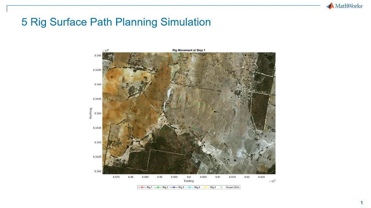
So thanks for joining us today. I'm going to start this presentation not with a PowerPoint deck, but to run some animations. And we're going to start off by looking at what's going on in the surface here.

So this is a rig path planning simulation. And we're looking at the final product of our environmental outcomes, where we're looking at the rig paths through our environment, which is designed to reuse existing assets and minimize the new production of pathways and pushing down trees and disturbance of rivers and dams and exclusion zones.

Next up, we have what we're going to do is our second use case here is we're looking at ore body simulations. And we're looking at doing smarter drilling programs than just meshed-out, grid-based drill approaches, where we're looking at using advanced statistical techniques to recursively push through and return sort of value decisions and reduce risk earlier in our situations. And what we're looking at on the left is the risk profile or the variance.

And on the right, we're looking at the ore body removing out. And this is a first-layer simulation. And we would normally then sort of recurse down to a second level, where we've now sort of outlined the rough shape of the ore body. And we now start to drill in-- pun intended-- and fill in the edges, fill in and refine the edges and the ore body block model through the interior.

So again, we're drilling to reduce risk. We're using our conditional simulation techniques to estimate risk or variance and target the drills accordingly. And this sort of rapidly returns value into the decision train earlier.

And then at a final simulation level, depending on the regulatory or investment requirements, we can use the same techniques to drill much further down into a much more refined mesh design for filling out block body models for life of mine planning. But again, we're using the same algorithm. We're using a conditional simulation approach to estimate where the next drill should go based on the uncertainty of the model.

Which, as a final product, leaves us with our three-dimensional view which we can explore and render. So we can imagine we have an ore body topper. We're looking at top of ore body in this case. We've got a fault running through the system, as well as some surface discontinuities. And we're just exploring that in relation to the overlying topology and topography of the landforms around it, particularly rivers, roads, existing farmland, and reserve or park land, which might have a higher environmental or different environmental constraints.

So that's the big teaser. Now let's just take a step back and have a look and work our way through how we can get to that process. So thanks for your time today. So the title of this talk is Optimizing Exploration While Minimizing Environmental Impact. And these are often sort of seen as sort of two different competing tasks. But I think we can work these through.

So my name's Peter Brady. I'm an application engineer in our Sydney, Australia office. I do work with a lot of our mining customers in Australia. And my core area of focus with MathWorks is in our maths stats optimization and cloud scale out in high-performance computing areas.

So what we're going to cover briefly today is sort of just walk through a big picture why are we here and then the data sources I've used in generating these workflows. And then I'm going to talk about the processes and the workflows for how we work through these. I'll, finally, outline some of the brief results we've got with some customers we've engaged with on processes similar to this.

So I'm really going to be focusing on workflows within our product suite. And I'm going to be illustrating these workflows, how we go through it with case studies. Now, these case studies are fairly neatly split into a sort of surface-planning component and an ore-body estimation component.

But I'd like to suggest to you that they're actually not really distinct in that respect. In that, because, realistically, one feeds into the other. We need to be able to get to the target locations to be able to drill, which becomes a surface-planning problem, which feeds into our ore body once we drill to then move into our next study, next sort of iteration of that process.

So just briefly, just conceptually, why are we here at the moment? So realistically and from the environmental context, at the surface level, there's an increasingly investor-driven focus on ESG outcomes, so Environmental, Social, and Governance. And there's clear benefits here from a customer or user mine perspective as well.

I mean, if we can minimize the environmental damage, be that water sources, surface water, sub water, tree cut downs, we can move into potentially lower regulation regimes and have positive environmental benefit outcomes at the same time. A big factor is a number of our customers really don't want to be the next front-page news item for agricultural impact. There's a fairly large created a lot of shockwaves late last year when, remarkably, ESG fail or cultural impact fail. And a lot of people don't want to be that. So if we can integrate these techniques into automation processes to avoid any cultural sites, then that's great.

So some of the questions we want to ask here is, given all that background, can we reduce the number of trees pushed? Can we drive out and design our roads smarter to minimize these impacts? Can we reduce surface water impacts by keeping crews out of creeks, out of watercourses? And can we eliminate cultural site incursions?

And on the geology side, we're really trying to maximize the return of data from our drilling programs. So oftentimes, within the industry, regular mesh drills are often seen as dumb and of limited value. But the flip side of that is they're often required for significant investment decisions to reduce and eliminate the risk on your ore body program for your life of mine, for your risk calculations.

So the question then becomes is if we have these two flip sides of the coin, on the one side, it's getting pushed back it's dumb. And the other, it's required by investments. Can we do it smarter? So can we do it quicker? Can we return usable data earlier to inform our design processes, right? Drilling programs take time. Drills are expensive. Let's see if we can do that quicker.

Can we drill fewer holes? And can we adopt a risk-based approach, right? So rather than just blindly drilling, can we use a statistical Monte Carlo-type framework or a risk-based approach to estimate probabilities of where our next drill hole should go. And does that allow us to reduce risk faster throughout the development-sites phase of a project?

And finally, as to why we're here, this is an intensely collaborative environment. People aren't working out here by themselves. We take data feeds, as part of this process, from geologists, spatial mapping specialists, and as well as the financials.

It costs money to run a dozer out through these areas. It costs money to send a drill team out. It costs money to analyze those drill results and part of that planning.

And then we have the producing team. And the producing team is really what we're targeting as the workflows through this talk here that I'm giving today. And it's how we can go through and use those data feeds, collaborate with those specialists to produce these plans, these paths, which are then, let's be honest, they're going to be consumed, at the end of the day, by our drill operators, who have to go out on site and hit those drill pads and get those targets for us.

They've got the dozer drivers and the road crews. We can load. We can load these path plans directly onto the GPS and greatly assist those dozer drivers to avoid flag areas and keep to the main path. They're going to be consumed further down the stream by our site management staff, who are over viewing those site construction schedules, as well as our resource schedules and mine planners. So we can get time estimates on how long these processes are going to take and what we hope to get back in the meantime.

So that's the overview as to why we're here. And let's just sort of now dive into those details of these workflows of how we get from these raw data feeds into those final visualization products that I showed at the start of this process. So data sources and processes.

Now, first up, I must acknowledge the data used from this. The data used in this demonstration is pulled from both the New South Wales Spatial Portal and Geoscience Australia. And it's predominantly SPOT satellite data and ELVIS terrain and elevation depth data. They're used under both creative commons by attribution and creative commons attribution licenses.

So this ore body is entirely fictional. It's based in western New South Wales roughly in relation to Sydney and some other significant deposits in the New South Wales region. There's a picture on the right here. As an interesting side note, this satellite image, which we're looking at here, was taken at the height of the drought in sort of early to mid 2020 before the catastrophic fires.

So if we took this image a little bit later, it would look significantly different. And as a little bit of a side note, there is you can actually see out in the middle of this photo, if you highlight where my mouse is, there is actually already some fire underway at this time, even in sort of Q1 2020 when the spot passes were taken through. But it is entirely fictional, completely made up. Any correlation with any known or to be discovered ore body is purely fictional.

And what data we're working with in this project? Well, we've pulled out the DEM rasters that are already available precalculated for it. We've also got rare raw LIDAR data, which has been flown for us on airborne laser surveys. And that's raw. We have to segment it. Can we use that to recreate high-res digital elevation models? Or is a five by five going to be good for us?

We're pulling satellite imagery and aerial imagery together to do advanced image analysis on this. So we're doing some deep learning, some semantic segmentation. And then we've got our GIS layers that our spatial teams are putting together for us.

So there are things like classified roads, tracks, rivers, dams, water courses, the places that we have to avoid and either avoid or, say, a cultural heritage site or a river to stay out of, or even places that we can use as a value to us, such as a road. So the existing, preconstructed road, nice, fast access point. We don't have to do any more work to it.

And then from the geology teams, we're pulling that exploration profiles. We're pulling ore body profiles, top depth down drill ore grade changes through that vertical profile. And they're all feeding together to produce an iterative loop towards the end where we refine our path plans, drill a target, and then, through the next iteration, refine our next particular targets as we move through.

So conceptually, I'm going to take the rest of this talk and split it out into surface and subsurface works and then bring it all back together at the end. In terms of surface work, this is the path we're focusing on here. So we're focusing on the DEM, the LIDAR, the satellite imagery, and some of the GIS layers.

So working through this systematically and through each of those layers, which we'll then join back together, the first one we're starting here is the LIDAR processing. And as rough reference, we're looking on the right-hand side image here. This is a picture of the raw, unsegmented point cloud. There's approximately 70 million points in there. And we're looking at an area of roughly four kilometers by four kilometers.

We can start to see hints of topology as we're looking at elevations scaled over from zero to one at this stage. Though, it hasn't been converted back to real elevations. We're just looking at point-cloud distribution. And we can start to see that there are sort of anomalies, which we would expect as sort of trees coming out and maybe some more vegetation type of our vegetation-type features.

So our challenge here is to segment this point cloud into ground versus nonground areas. We then have to do feature extraction and classify down to Australian standards, promulgated by the ICSM or the Intergovernmental Committee on Surveying and Mapping, which essentially lays out point-cloud classification. So say for point of argument, classification one is ground. Classification five may be vegetation and so on.

And how we do that is we work from our raw point cloud. And the first process here is to really apply a morphological filter to split the ground to the known nonground points there. And this is based on an implementation in the LIDAR toolbox. And it applies a simple morphological filter published by Pingel et al in 2013.

And this segments out into the ground. And then we've got these two little helpers here. And the two little helpers is a two-step tunable process where we segment those extracted features.

And what we do is where really the first path is extract features is really computing things like normal and curvature algorithm on clusters of spatially related points. And this gives us these sort of curvatures. And the normals give us indications of how curved that work points in that region, that surface in that region might be or how flat it might be.

And conceptually, why we do this is because nature doesn't build straight lines. Curved features are generally trees, shrubs, bushes, natural-type features. Whereas buildings tend to be flat, to have straight angles. The points in the neighborhood are sort of correlated in a plane with consistent, normal directions.

And that allows us, through those two steps, to, first of all, split out into sort of the building versus vegetation points. And then once we've got those vegetation points, we can quite easily split them into sort of low and medium and high vegetation based on our point cloud from ground. And we just do sort of a correlation difference between adjacent ground level and the top of the point cloud that that vegetation is on.

So how do the results look for that? Well, we're looking at a map view of our site here. On the left is the raw aerial photo. And on the right, we're looking at a scatter plot of the LIDAR pings, which has been classified as high vegetation points.

And in general, for the high vegetation points, it's doing a very good job. We can do a quick just a left to right comparison. And I'm very happy sort of with that is picking up the results.

At the other extreme, though, we really want to look at also the low vegetation. So while we're focused on trees, we do want to try and minimize our shrub push downs as well. And in this case, the results are perhaps not as good as what we were expecting.

It's because we're sort of seeing some broad areas of low vegetation throughout the middle. We're also seeing some suspiciously sort of straightish lines within this process that I wouldn't necessarily be expecting that aren't correlated with any sort of topological features over on the left-hand side. But to be honest, I'm highlighting this because it comes back to an understanding of our physical quantities that we're measuring.

When this survey was flown, this is the low vegetation is defined as less than 300 millimeters above natural ground. We're really sort of bordering at the noise level of the LIDAR ping at this point. So we sort of have to take this with a little bit of a grain of salt and just be happy with the high veg. Medium vegetation is pretty good. Although, I've not shown it. And just take with a grain of salt the low vegetation, as it's going to be an awfully close to the noise signal coming out of our LIDAR.

Now, just as this is quite a computational and RAM-intensive algorithm, so I batched these out. And it used 350 to 500 gigabytes of RAM to batch all these out as a one-pass process of all 70 million points. So that's how we've pinged out the LIDAR and had a quick look at it.

So moving on to semantic segmentation, now, semantic segmentation is the process of applying a deep learning model to images to classify the individual pixels within that image. So our goal here was to take our satellite images and be able to classify into paddocks versus tree vegetation. So we're providing sort of a stop-gap background here to fuse data between both the LIDAR and the satellite imagery. Because we may have sites where we're fortunate in this case where we have both aerial imagery and LIDAR.

So I was able to reuse a fairly standard network topology that's quite easy to create within Matlab. You can see, for the deep learning people, the network that I used over on the right there. I ended up training this on a parallel CPU network. It took about three hours, required about 140 gigs of RAM. I was pushing raw satellite images, which are approximately 1,500 by 2,200 pixels and a little bit too big for a GPU just to push those raw pixels through.

I followed a fairly standard image labeler workflow here, where I used the image labeler app. And the flood fill feature was fantastic in this case. So I was able to click in the middle of paddocks and rapidly label areas of similar color. And you can see an example over on the right here with the blue areas is sort of the more agricultural-based sites. And the red is highlighting the different trees that we wish to segment those pixel classes into.

I was able to segment. Sorry. I was able to label 16 images, 2,200 by 1,500 pixels in less than an hour using this app technology. But this does come with a caveat. Like all deep learning models, it's only as good as the images that the model is trained on.

So in this case, the caveat I have to add is I was training these images on images taken at the height of the drought. Now, I can guarantee that I will have to retrain this model if I was to redo this work today because the drought's broken. Most of these little dams on the right here that are not visible because they're empty. They're just dirt at the moment. And they'll be full. They'll have water in them.

And the ground over here will be green. The trees will be a lot greener. The paddocks will be a lot greener. So I'll have to completely retrain these models for the terrain now. And that's a fairly common deep learning path.

So again, how did we work out? Well, we can see over on the left here, again, we're doing a left-right A-B style type test. On the left, we've got our raw site. And on the right, we can see a couple of things first up.

At the northwest quadrant, we're doing really quite well. We can just do a qualitative comparison. And we're pulling out the trees and the shrubbery mostly, as we expect. Similarly, moving down through west and the south, in the south, we're picking out all the trees as we would expect through the reserve area.

Now, interestingly, over on the right-hand side here, where we can see we have quite a different soil profile, different colored soil profile, we're overestimating the number of trees present on site. And I'm happy to accept that for this model at this stage because I'd much rather have-- the purpose of this model is to minimize tree damage. So I'd much rather have a conservative overestimation than underestimation in this case. But and this is sort of one of the importance of data fusion, that not each data source is going to be a whole source of truth, as we're automatically processing like this. So that's the data segmentation and semantic segmentation that we can use for this tool.

So the final raw data source we have is our GIS layers. And we pull them directly from our shape files produced by our GIS team or our special mapping team. And they allow us to extract designated features, such as rivers, dams, creeks, roads, or tracks, cultural sites, and existing cadastre.

Where are my property boundaries? Who am I going to have to apply to permission to access? And we allow to set buffer zones on those. So say if we're running quite a large dozer down here, it might have a sort of a five to seven meter blade on it. So let's set 10 to 20 meter buffer zones around cultural sites. Let's set 20 meter buffers around rivers to keep our team try and minimize the impact on the water courses.

But on the flip side, let's promote our roads and tracks. And let's use those existing road and infrastructure to our advantage to minimize our site work. So we can reuse that content, reuse that already in place. Massively speeds up our time because we don't have to do-- it minimizes our construction costs.

So that's the final piece in this raw data puzzle. The next thing we have to do really is to actually just bring it all back together before we actually do that path planning. And what we're using here is we're using a mesh of possible paths. And then we're using some graph theory.

And graph theory is used in a lot of different things. Like the most common place graph theory pops up is network connection. So you and your friends on LinkedIn can be modeled by a graph, where you're a node. Your colleague is a node. And your connection or your friendship between them is the edge.

In this case, though, what we're doing is we are using those existing algorithms. There's a lot of mathematical theory already around about graph theory. And we're using sort of what we're calling what's a weighted shortest path.

And the weight, in this context, is interpreted as the cost to move over that node. So existing tracks and existing infrastructure has an incredibly low cost to move over that track. So the shortest-path algorithm prefers to use that.

Coincidentally, if a node crosses a creek, or flip side of that, if a node crosses a creek, that has a very high cost associated with that because we want to minimize the creek crossings and maximize the reuse of existing bridges and infrastructure. So we set up this weighting system where we fuse the data from the GIS. We fuse the data from the semantic segmentation and the LIDAR to come together and segment to create this weighting.

And the key part of the weighting here, though, is, once we have created new tracks-- and there are cases where we're going to have to. We sometimes just have no choice. If we need to get to that drill, we have to push those trees down. But the key part of this iterative approach is, once we've created those tracks, we reset the weights on those nodes, so that we can reuse the algorithm. We'll prefer to use those tracks again in the future rather than constantly creating new tracks wherever possible.

OK, so that's the completion of the surface work. Conceptually, that's the ballpark. And what we do is that we use these data to set up the path. And then we use that hand in glove in an iterative procedure with the subsurface ore body works.

OK, so that brings me neatly through to the subsurface ore body works. So we're focusing on the geology and the conditional simulation at this point. Now, what that means in practice is we're using an established geologic technique called conditional simulation.

And we fit sort of a Monte Carlo approach here, where we fit a couple of different simulations in this case. And we look at the differences in the variances across those simulations. And where the simulation is in high agreement, the variance is low. And where the simulations are quite different, the variance is high. So we can correlate variance very highly with risk.

So we can see the picture on the right here is an example of halfway through the time-step simulation. And we can see the green crosses. The green crosses, particularly out around the outside, are targets that we've already drilled and already know about.

The black dots in the middle is mesh that we have to get to. So this is a first-path level. This is our first-level recursion. We're looking for ore body shape definition here.

And what we're looking at is the colored surface overlaying the aerial photo is our variance. So the yellow areas are the high, where the conditional simulation has a lot of uncertainty. So that's where we have a lot of risk. Really, we don't have a lot of confidence in what's going on there.

And that's how we're targeting our next drill. So we can see the green stars just highlight over the top there, our next drills that we're going to hit. And for this particular simulation, the drill targets were picked to reduce that variance as quickly as possible. So at each iteration, they're the top five variance locations. But these can be tuned. These location selections can be tuned to, say, find edges quicker or move into a sort of different priorities that you may need for a particular simulation.

But a final point I want to run is this simulation is based on the top depth of the ore body. So we're interested in rapidly finding the depth of the overburden. However, we've worked with a number of customers. And we can extend this to multiobjective simulations.

So we can, simultaneously, look at top of ore body, bottom of ore body, grade profile of different ores throughout the drill profile. So it can be extended to a multiobjective simulation. So that's the general process for a conditional simulation of the ground.

And now what we have to do is just bring this all together into sort of one cohesive package, if you like. So what we do is-- coming back to this data, the surface work, this data flow program is we are looking over on the right-hand side of this picture. And it becomes an iterative loop.

Our conditional simulation we use to target or generate those next targets for the drill, which feeds into our path plan, which is then drilled. And as the results from the drilling team come back, we, first of all, reset the paths that we had to create to recognize that we have some new tracks in place. After the drill, we rerun that conditional simulation to generate the next path and so on and so on.

So that should add a bit more context to those final animations, those first animations that I showed right at the start. So to add some full context before I run it again. So the final operational simulation that we're working with here, we have five drill rigs.

We are starting with 15 preknown survey points. And the challenge here is to use the data to minimize the path of least impact across the surface. And because we've got five drill rigs, we are going to be iterating five targets per time step.

So with that context, so again, keep an eye on what's going on here. On the right-hand side, we have the top of the ore body. These are in HD, standard data. And on the left-hand side, watch as the drill bits approach.

So we have our known drill starting out. And we're going to drill through this simulation as we go. So we can see the variance in the simulation starts relatively high. We have the high uncertainty areas around the edges. We have a fair bit of confidence towards the middle of our simulations. But as the simulation and program progresses, that value changes.

So there. We've done the first-level recursion on the left-hand side. We've drilled out all the points that we need to at this stage. And we have a rough understanding of the outside of the ore body at this stage. The funny little triangulation here is just an artifact of the triangulation approach to visualize a relatively coarse mesh. As I showed at the start, we would target a second-level drilling campaign to refine this edge and the shape of the ore body.

But how did that look from the surface? So again, to provide a little bit more context to what we've already seen, we have our five rigs starting atop of each other. So this is our access point, the closest point to the major bitumen road, quickest to get our infrastructure in.

There's also, as a point of asset, there is a existing track structure running across the top of the ridge, up the ridge and across the top of the hill through to easy link up with our roads on the southern side of the sector. And we already have two bridges in place. So this is, strategically, a very good starting point for running this simulation because we have good access to bitumen roads. We've got existing infrastructure and creek crossings. It minimizes our construction costs.

And again for context, we're starting this simulation with our known drills. And I think the thing that I'd like to highlight as we're watching this is it flashes through a little bit quickly. So I'll probably run it through a couple of times. But as we're watching, we can see that main central route is used a number of times. And this is a good example of that path-planning algorithm, trying to reuse as much of our existing ease-of-use access recharging infrastructure to minimize reconstruction costs.

So finally, in conclusion, bringing those all together, this demonstration, this work was inspired and extended for some work and proof of concepts we did with a customer. That customer, at the moment, has this program in place and is underway and using it. They're expecting a sort of a 70% reduction in tree damage, up to a 40% reduction in low vegetation. And they were looking to eliminate cultural site incursions. We're hoping to get a user story from that customer later this year as the results of the program come through.

Now, just as a quick highlight here, I used quite a lot of different tools across our product suite here. So I used our core computer vision image processing and LIDAR toolboxes for processing a lot of that, preprocessing those aerial photos as they came through, preprocessing and segmenting those LIDAR clouds and those point-cloud data that comes through.

I use the mapping toolbox to generate those plots and pull data off different GIS and web servers. And then finally, a lot of the grunt work was undertaken through our stats and machine learning toolbox and deep learning toolboxes to actually do the grunt work of the statistical and mathematical models underlying those graph theories and moving, merging those weightings together for the path planning.

I did mention I burnt a lot of compute time out on AWS for this. The conditional simulation is computationally intensive. But we're talking order of magnitude or running a computation overnight for the entire 50 simulations. So it's very compute effective to run this in terms of a drill program, where it might take days or months to analyze different drills.

I didn't use GPUs for training this particular image data set for the semantic segmentation. But the GPU training facilities for the semantic segmentation can be incredibly effective. Finally, parts of the system identification toolbox we used in the conditional simulation package.

Now, I want to highlight here that this might seem like a big and deep toolbox structure. And plumbing these all together is quite difficult. But that's the real power of the Matlab environment is that these all sit together. They use common data structures. And it's very easy to plumb these straight together. There's no mucking around with dumping to external data or bringing it back in. It's the integrated unified data set.

So look, thank you very much for your time. I hope you've seen this as a bit of an inspiration and something that can inspire you to say, how can I use this for your work? And if you're interested, I encourage you to contact us for assistance.

So we have application engineers like myself. And my role is to generate proof of concepts like this to work with you to see how our tools can be used to accelerate your workflows. We've got training services to rapidly upskill you in the use of these products. And we have consulting services to drive your engagements collaboratively with you to rapidly return investment on your projects.

Because, at the end of the day, you successfully using our products is how MathWorks achieves success. So please contact Wilco or myself if you're interested. And thank you very much for your time in this presentation.