Optimizing Solar Array Performance Using MPPT
Learn how you can model and analyze a photovoltaic system using Simulink and Simscape Electrical to achieve maximum power output. The model uses irradiance, solar cell, and boost converter models to simulate the system for 24 hours. Maximum power point tracking (MPPT) using impedance matching is explained as a means to drive the systems to provide optimal power for changing impedance.
Tadele Shiferaw is an application engineer at MathWorks Benelux based in Eindhoven. He coordinates the engagement on power electronics design and control with customers from multiple industries within the Benelux area. His technical focus areas include physical modeling of systems, controller design, systems engineering, and hardware-in-the loop simulations. Tadele completed a graduate study in control systems and a PhD in controller design for safe robotic manipulation at University of Twente in the Netherlands.
Published: 15 Jul 2022
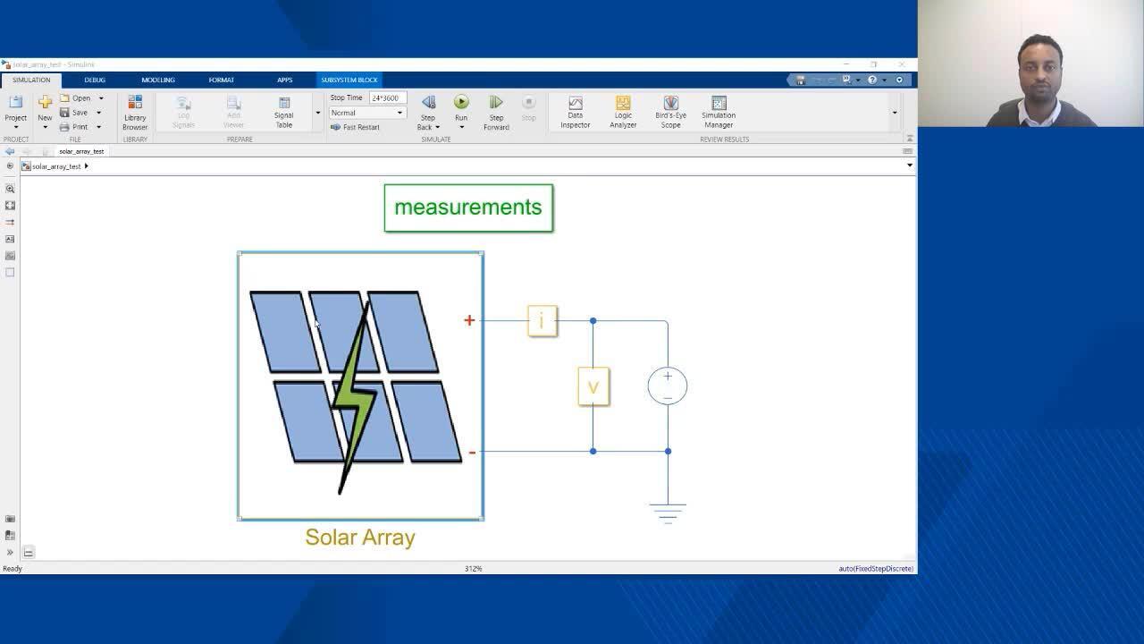
Here, I have a lexical model of a solar array connected to a load. And I can use this model to run multiple simulations to validate the performance of the solar arrays. If I explore what's under the hood, I can identify three main components. So the solar cell and two additional extending components here.
The major component of the solar cell, is the block that converts the irradiance or the power from the sun into electrical energy that flows through the rest of the system. While we are defining the cell behavior here, in the configuration, we can also define how a number of these cells could be connected either in series or in parallel to create a panel or an array configuration.
While this manual parameterization is a possibility here, there is also an option to actually select a manufacturer, and then also a part number so that there is an automatic parameterization based on the data obtained from manufacturer datasheet. Once we parameterize the solar cell, we have to extend it with additional components, MPPT, and a boost converter that we'll discuss shortly. And then finally connect it to a load so that you can create a performance simulation of a system.
Here in this case, I'm running a full simulation for 24 hours using the solar cell. And then I'm also capturing important measurements that I can inspect afterwards. For example, I can check the maximum power that I was able to generate from the system, and then the power that was consumed by the grid, which was obviously less than the solar power. Then I can also look at the voltage and the current that was produced from the solar cells.
The reason why we have those two additional components, the MPPT and the power converter connected to the solar cell, is because of its special characteristics captured in this IPV curve. The IPV curve, which shows the output voltage versus the output current and the output power, shows that the current deteriorates sharply after a certain threshold voltage.
That means that the power gradually increases towards a higher maximum point and then also gradually declines. If we need a very efficient operation of the solar cell, then it means that we have to drive the system to operate at this maximum peak operating point.
And one thing to note here, is that because of changes in ambient conditions, like temperature, or the solar irradiance, this whole curve could shift up and down or left and right. So it means if we need a continuous operation at that efficient point, we have to continuously keep track of where the maximum power point is, and guarantee that we are driving the solar cell at that operating point.
The whole operation of this maximum power point tracking, is implemented by using a concept of impedance matching. Impedance matching is a standard electrical engineering concept where if you connect a source to a load, maximum power is consumed by the load when the impedance of the load is equivalent to the impedance of the source.
So this ideology is applied to design the MPPT algorithm, and that is demonstrated by a model here. This model contains two different system implementations that I want to compare using simulation. Both systems contain a constant DC source, and then they have a similar impedance implemented as a resistor.
Both systems also contain a variable impedance load implemented as a variable-voltage load here and here. You can see that the main difference between those two systems is, the second system contains an MPPT algorithm implementation together with a buck/boost converter so that we deliver maximum power to the load irrespective of its impedance.
So let's run a simulation here and then compare the power delivered to the load in both scenarios. So the simulation is complete. And I can inspect what happened there. So, for example, on the first case, I can look at the power. And then you see that the power was varying and it varies depending on the impedance of the load.
On the second case, I can look at the power consumed, and then you see that the power almost maintains a constant value of around 100 watts, which has also delivery at 100 watts throughout the full simulation cycle.
And then if you want to check the second case, you see that the variable voltage on the load side, which means there was a variable impedance also implemented on the second side. But irrespective of the impedance side on the load, we are able to deliver this maximum 100 watt output on the second circuit versus the first one. So that was the value of the MPPT algorithm together with the converter.
Related Products
Learn More

Featured Product
Simulink
Up Next:


Related Videos:


Select a Web Site
Choose a web site to get translated content where available and see local events and offers. Based on your location, we recommend that you select: United States.
You can also select a web site from the following list
Americas
- América Latina (Español)
- Canada (English)
- United States (English)
Europe
- Belgium (English)
- Denmark (English)
- Deutschland (Deutsch)
- España (Español)
- Finland (English)
- France (Français)
- Ireland (English)
- Italia (Italiano)
- Luxembourg (English)
- Netherlands (English)
- Norway (English)
- Österreich (Deutsch)
- Portugal (English)
- Sweden (English)
- Switzerland
- United Kingdom (English)