Optimizing the Design and Operation of Radar and Antenna Systems in MATLAB

[AUDIO LOGO]

Hello, and welcome to our talk on optimizing the design and operation of radar and antenna systems. Before we dive in, let me introduce myself. My name is Sumit Garg, and I'm a senior application engineer at MathWorks' India office. I've been with MathWorks for around four years now. Prior to MathWorks, I spent seven years in development of radar software applications in aerospace and defense industry.

And my name is Chris Lee, and I'm the senior product manager of our optimization products. I've been working with aerospace and defense and automotive companies on design optimization applications and capabilities for about eight years, and I'm based in Boston.

You can also check out what others are saying on social media and share your excitement using #MathWorksExpo. We would also love to connect with you on LinkedIn.

So thank you all for attending this session. We will start the presentation by describing the motivation for design optimization for radars, then we will show you three use cases of optimization to satisfy the design objectives. The first use case is to optimize the resource allocation for a multisector surveillance radar.

Then Chris will present the second use case, which is using optimization for beam pattern synthesis. And we will then present an antenna design optimization workflow. This will enable you with system level to component level design optimization. We will conclude the webinar with a summary and more resources that are available to help you with radar design optimization projects.

Multifunction Phased Array Radar performs multiple tasks, including searching for the target, tracking them, classifying the detected target, communicating with the other systems, or protecting against interferences. Having a phased array front end provides agility in beams steering and switching between different beams. These functionalities are usually multiplexed, not only in time, but also in angle.

And each of these functionalities requires certain resources, such as signal bandwidth or the beam width. And we all understand that there are several constraints on the available resources. Therefore, it is important to be able to model a system that performs different functions and find the optimum resource allocation for these functionalities in different conditions.

Also, with growing number of connected devices, the frequency spectrum becomes increasingly congested. To make the frequency spectrum usage more efficient for radar communication coexistence in the radar and the communication communities, you can optimize the desired beam pattern to avoid transmission to or reception from certain directions to mitigate against interferences.

For example, we see in the recent news that deployment of 5G system in the C band has caused concerns for interfering with radar altimeter performance, which is a safety-critical flight instrument.

Besides the interfering challenges, another radar design challenge is resource allocation. For performing multiple tasks, there are limited amount of resources available. These resources can be in the form of bandwidth, transmit energy, time budget, or maybe the computation resources available on the system.

You want your system to allocate the available resources in a way that the mission of each function is satisfied. Antenna design is another part of the radar design that can benefit from optimization workflows. This can include minimizing the antenna size while maintaining the impedance matching and maximizing the antenna gain.

You can address these challenges with optimization workflows in your modeling and simulation. First, you need a platform that you can model and simulate different parts of radar system with high fidelity at different abstraction levels. For example, to optimize the resource allocation, it is critical to be able to model a closed-loop radar system, including the resource management and controls block.

You define the initial design parameters, constraints, and the objective. And based on the problem definition and the desired output, you choose a proper optimization solver.

The optimization solver starts with a set of initial design parameters and modify these parameters till the design objectives are met and the optimal design is achieved. With optimization workflows, you can find optimal designs, reduce design iteration time, and automate operational decision-making.

With this, let's introduce the first example of resource allocation for multifunction radar. The search-- task quality, or the probability of detection, is a function of power of aperture product, which is defined as the product of peak power and the aperture size.

On the right hand side, you see the probability of detection for each search sector for different target ranges. The larger the power aperture product, the higher the probability of detection for a given target range. Therefore, a larger power aperture product implies better detection.

You can also see that each search sector needs different amounts of resources to maximize its probability of detection. And that depends on the search frame time and search volume. To quantify the search task quality, let's define the detection range where the probability of detection reaches 90%. This is shown by a horizontal black line on the right-hand side chart.

Here, you see the detection range for different power aperture product resources across different search sectors. The dotted line showing the range limit for each search sector. Note that the search task quality is increasing by increasing the resource or the power aperture product. At some point, the detected range does not improve any more with more resources.

Now, let's assume that we have unlimited power aperture product available and define our set of objectives' detection ranges for each search sector using fmincon function, which is a nonlinear optimization solver. You can find the required resources for each search sector to reach the objective range.

Now, on the right-hand side, you see the coverage of different search sectors in normal operating conditions. The bar graph on the far right is showing the amount of resources allocated to each search sector. The dashed line on the chart in the middle shows the achieved radar detection range for each search sector, given the allocated power aperture product.

Now, the question is, what if we only have half of the required power aperture product? With quality of service optimization, you can optimize the search quality by maximizing the weighted sum of utility function across all search sectors. But what is our utility function?

In previous slide, we saw that the detection range is a function of power aperture product. And here, the q is the detection range for search sector, given amount of power aperture product. The utility function describes the degree of satisfaction with how the search task is performing.

For each search sector, besides the objective detection range, you define a threshold detection range. You can see that, when the detection range is increasing from the threshold to objective detection range, the utility function or the degree of satisfaction with search task is increasing.

The joint utility can be maximized by first weighting and then summing the utilities of individual tasks. This is important to avoid unfair resource allocation. Let's look at the resource allocation for when we have only access to half of the total power aperture product needed to satisfy each search sector objective detection range.

We give the horizon sector the highest priority and the long-range sector the lowest priority. And for the initial values to start the optimization with, we distribute the total power aperture product available between three search sectors. On the bar graph on the far right, the first thing to notice is that the total power aperture product has been divided in half.

You can also see that the horizon sector has got the same amount of resources as before, while the resources allocated to the long-range sector has decreased significantly. You can also see on the graph in the middle that the detection range for the long-range sector is the farthest from the sector range limit compared to the other two sectors.

In summary, with quality of service optimization, you can find optimal resources allocation to satisfy the mission across all different tasks. And with that, let's move on to talk about using optimization workflows for beam pattern synthesis. Over to you, Chris.

So we just saw how you can optimize radar resources across multiple search sectors. Searching each sector requires scanning across a search grid with targeted beams. And this is performed using a phased array of antennas. So in this section, I'll talk about how you can apply design optimization to array beam pattern synthesis.

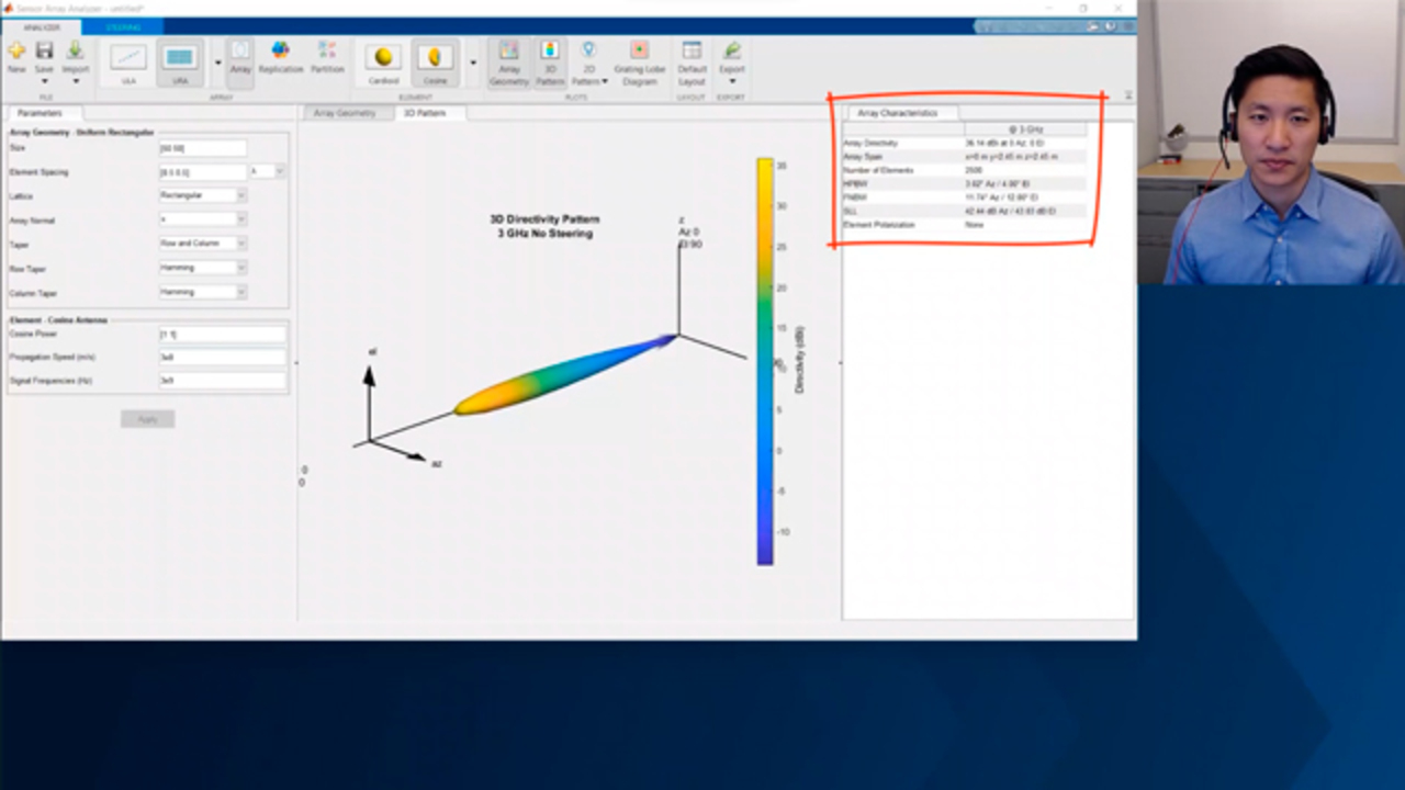
To get an idea about the types of parameters involved in phased array design, let's take a quick look at the sensor array analyzer app, which enables you to construct and analyze common sensor array configurations. So we'll start by selecting from a set of 2D or 3D array layouts and choose the type of antenna element for our modeling.

And then we can plot the 3D directivity pattern. In this case, you can see that we don't have great directivity. But we can then go ahead and modify multiple parameters that define the array geometry, including the size, element spacing, and other parameters, as well as modify parameters associated with the antenna elements.

And then, of course, each of these modifications will affect the performance of the array. So we could look at the updated 3D pattern and see that we have achieved better directivity, as well as analyze the array characteristics.

Now, massive MIMO arrays may include hundreds or even thousands of elements. And given all the different design parameters that you can modify, it can take many iterations of manual trial and error and, really, a lot of time to arrive at an array architecture that achieves a specific pattern. So how can you design an array that meets the specific requirements of your system?

Well, this is where design optimization comes in, optimization takes the guesswork out of the process and automates the search for an optimal design, resulting in more performance and sometimes even nonintuitive designs all in less time. Now, given an initial beam pattern, you develop a cost or objective function that defines the desired pattern attributes, along with any constraints that need to be considered.

And then the optimization solver will automatically iterate through different design parameter combinations to move toward that optimal pattern. So let's take a look at an example.

We'll assume you're determining the weights for a 32-element uniform linear array, but you can apply the same concepts to any array geometry. Earlier, Sumit talked about interference challenges for radar. So let's consider interference here.

The signal of interest is at 0-degrees azimuth, but we also need to null out interferences at three known locations. It turns out that there's an approach called linear constraints minimum variance beamforming, which provides an optimization formulation that will minimize the total noise output while preserving the signal from a given direction and nulling out interferences from other specified locations.

And, in fact, you can compute a closed-form solution to this optimization problem. You can see in the beam pattern graph how the signal is preserved at angle 0, and the noise sources are eliminated in the direction shown by the vertical dashed lines.

But another common requirement for pattern synthesis is to ensure that the response is below a certain threshold for a set of given angles. So, for example, the dashed lines now represent a couple additional upper limit constraints we're adding on the side load levels for different angle ranges. And these additional requirements introduce inequality constraints in our optimization problem. And so a closed-form solution is no longer available.

Thankfully, the phased array system toolbox provides a new and really convenient function called MinVarWeights, which automatically uses numerical optimization techniques to compute the minimum variance weights to satisfy the requirements. Now, under the hood, the function uses a second-order cone programming solver from the optimization toolbox. And without this function, the user would need to go through a pretty complicated formulation to use the solver, and this is still shown in our documentation.

But with this function, the user just needs to provide input, such as the element positions, beamforming directions, and some other optional inputs. And then the function will provide the optimal beamforming weights.

So the plot shows the resulting pattern, which satisfies these new requirements and provides good sideload suppression. Now, we focused on optimizing the weights here, but these same types of workflows could be used to design the positions of antenna array elements, for example.

Now, we just considered an example where the beam was directed toward a single direction. But in radar search and track applications, the beam direction is not static but is modified to sweep across a range of angles to cover the search grid. You can apply minimum variance beamforming to meet changing pattern requirements while beam sweeping.

So to see this, we'll consider a new situation with some different constraints. Here, the sideload levels must be less than a tapered sideload mask, as shown in the plot, and there are interferences at four locations that require nulls.

So as before, we can use the MinVarWeights function synthesize the beam pattern. That will minimize the total noise output and satisfies these requirements. We've directed the beam at 25 degrees in azimuth.

Now, if you need to sweep the green-- if you need to sweep the beam across a range of angles, you can simply call the function iteratively. The resulting pattern covers the required angle range, while satisfying the adjusted sideload level requirements and maintaining the nulls at the interference locations.

All right, so we've seen how you can apply optimization problems to solve problems involving radar operation and phased array beam patterns. But you can also apply optimization at the component level for antenna design. Let's take a look at an example.

So you can perform the antenna design optimization workflow directly in the Antenna Designer app. This app lets you design, visualize, and analyze antennas interactively. And in this example, we'll consider the design of a fractal island antenna, but the same workflow can be applied to many other types of antennas available in Antenna Toolbox.

So here we see our initial antenna design with the input parameters defining the design shown on the left. And then given the design, we can analyze the performance characteristics, such as the impedance, the S-parameter and the directivity pattern. This current design is resonant at 2.4 gigahertz.

And from the results, we can see that the impedance matching and the bandwidth of the antenna are not very good, and the antenna directivity is just 4.6 dBi. The area of the antenna is about 30 centimeters squared, which is too large. And so we want to minimize the surface area of the antenna while improving its gain and bandwidth performance.

And this is not easy to achieve via manual trial and error, given the many different design parameters to consider and the multiple requirements we need to meet at the same time. And so we'll use the optimization capability directly integrated in the app.

We'll first select our objective function. In this case, we want to minimize the area of the antenna. And then we can select the variables of the antenna that we want to include in the design space. For each of these, we have to provide a minimum and maximum bound value.

And we can look at optimizing geometric properties, as well as material specifications, and even lumps element values. But in this case, we'll just focus on optimizing the shape of the antenna. So the design variables we select are the length and width of the antenna, of the slot, and of the ground plane. And we set appropriate lower and upper bounds for each.

Next, we'll define the performance constraints. The current design has a gain of 4.6 dBi. And to improve this, we set a constraint so that the gain is greater than 8 dBi. And then we'll add an additional constraint for the S11 to be less than negative 10 dB.

That we keep the center frequency at 2.4 gigahertz, but we can change the frequency range to include fewer points so that the optimization runs more quickly. And then as a final step, we can increase the number of iterations to 300, as well as enable parallel computing to speed up the optimization.

Now, the app offers surrogate optimisation methods, which are well-suited for these types of expensive, simulation-based optimization studies. But the process still takes a bit of time, and so we'll skip ahead to the end of the optimization solve.

So now we can see from the convergence plots that the optimization has completed the full set of iterations. We can go ahead and accept the results and verify that the antenna performance of the optimal design is what we want.

So as you can see, the antenna is still resonant at 2.4 gigahertz. And the S11 behavior has significantly improved. The directivity of the pattern has also significantly improved and now has a gain of more than 8 dBi.

From here, we can further refine the design by changing the material from a perfect electrical conductor to copper, for example. Overall design optimization has significantly improved the results on all fronts, and we have an antenna size now of smaller than 8 centimeters squared.

Now, this same integrated optimization workflow that we just saw in the Antenna Designer app is also available in the Antenna Array Designer and PCB Antenna Designer apps. So from each of these apps, you can launch an optimization study, and the apps provide objective functions and constraints specifically for array and PCB antenna optimization.

If your optimization problem requires a configuration that's more complex or customized than the one allowed by the app, you can define your own customized objective and constraint functions and then use any of the methods provided by Optimization and Global Optimization Toolboxes. Our documentation provides examples showing this custom workflow, including the ones shown here.

All right, so with that, let's just wrap up with a quick summary and some resources. So we've seen that the complexities of multifunction radar systems and 5G systems are driving many technical challenges and requirements for engineers. Many of these requirements can be formulated as design optimization problems.

You can use MATLAB to model and simulate these systems and then use an optimization solver to automatically explore the design space and identify the optimal design for your requirements. You can apply these types of workflows from macro- to micro-level decisions or, in other words, from system-level operation to component-level design.

Using design optimization that allows you to automate operational and design decisions. You can reduce the time to explore the design space and find optimal designs that satisfy complicated requirements.

Of course, this was just a quick overview. So we've got plenty of additional resources available so you can go deeper, such as Tech Talk and workflow videos. We have free and instructor-led training courses and detailed documentation examples.

And, of course, please reach out to us if you're interested in learning more. With that, that ends the talk, and I'd like to thank you for joining. Thank you.

[AUDIO LOGO]