Pricing Weather Derivatives with MATLAB
Pricing a weather option involves getting a good model for the climate event. Learn how to price a weather option using the following steps:
- Get data into MATLAB using a REST API.
- Clean and analyze the temperature timeseries.
- Model the temperature using a linear model for the deterministic part and an arma/garch process for the volatility.
- Forecast the temperature and price of a weather option.
Published: 12 Oct 2021
In this first example, we're going to show you some of the steps involved in pricing a weather derivative. The main idea will be, however, to show you how to get climate data into MATLAB, and then how to process it so that it can be used in financial applications afterwards.
Now, first of all, let's very briefly describe what is a weather derivative. This is a financial instrument product used to hedge against the weather. And the idea is that the seller agrees to bear the risk of an extreme weather event in exchange for a premium. It works very similar to insurance, with the difference that you don't have to prove your claim in order to get paid.
Now, there are many types of these weather derivatives. And for simplicity, we're going to focus here on one which is based on the accumulation of heating degree days. I think the degree day is defined as those days where the average temperature falls below a certain amount, which typically is set as 18 degrees.
And the idea is that on those days, people would tend to turn the heat on, and therefore its name. The idea is that during a year or during the period set in the contract, you can accumulate how many degrees you fall each day below this 18-degree mark, and then accumulate that for a period of a year, or whatever the contract duration says.
Now, once you have this number, the way to price the option is as follows. You have a strike level, so the amount of degrees below which you don't get paid. And then, above that, there's a dollar per degree, where I would define the actual price of the option.
This is a very simple equation. And the interesting thing is that the only thing you need to price or to forecast the price of this option is the actual average temperature during a year on a certain location. So that's what we are interested on, getting the temperature and model temperature in a location over a period the next year or the next two years.
Now, first of all, where do we get temperature data? This is the first option that we'll have to answer. Now, you'll find many different places and many different websites, many different institutions, providing data.
In this case, we're going to use the NOAA, or the oceanographic and atmospheric center in the United States. Most of these institutions that provide data will normally provide it via what's called a REST API. And in case you're not familiar with it, the idea is that they'll provide you a set of URLs or links that you can use to download the data directly into MATLAB.
So how does this work? So typically, you'll have to authenticate yourself. And in the case of the NOAA, when you register with them, you will get a token. Then, to make a call, you will need the URL, which is basically the endpoint or the address of the data that you want. You will need your token, as you see here. Mine is blocked now, but you'll have a set of passwords. And that's it.
And then the way to get the data is simply make a call called data=webread, your URL, the options, in this case, that you have fill with 'token', and then any additional options, if any. And then typically, the external website or service will tell you what different URLs you can use to call your data.
So in this case, for example, you can see that I can select the different stations or different locations where I have available data. And I pass it a coordinates option to define where we actually want the data. In this case, I'm looking at somewhere near Stockholm, and I see that there's three different stations, providing data. And I see the minimum date, the maximum date, where they are, the name, and whatnot.
And then I can do the same for data. In this case, you see that my call is a bit more refined. I know what type of data I want, which is daily data for average temperature. I know the dates, the units, and whatnot. Once I get the data, the first thing I can do is I can actually plot the data in that. For example, in this case, I'm getting the data for the year 2020, in this station near Stockholm. And then I can plot the data and I can see the cyclical value of the temperature, so colder in the winter and hotter in the summer.
So you see it's quite simple. In the end, the REST API is just a URL. And then you use the functions, webread and webwrite, in order to make separate calls to them. If your call is a little more complex, MATLAB has a Http interface that will help you add the complexity of the call. But for most simple cases, or for the vast majority of cases, webread and webwrite will be enough.
So let's go now into how to actually process and model this data. Now, once I have loaded them to MATLAB, the next step is to actually model the temperature or the upcoming temperature for the next years, in order to have an idea on how much this option will cost. Now, for this, I have a file with some preloaded temperature from 1978 till the end of 2020. You can see here. And the temperature is collected at the same location that you saw above.
Now, the first step is to check that-- I need data for every single day. So I'm going to check that I have all dates covered. And by doing that, comparing the height of the table to the total number of days between these years, you see that they have a deficit of 70 days, where the API then gave me the data.
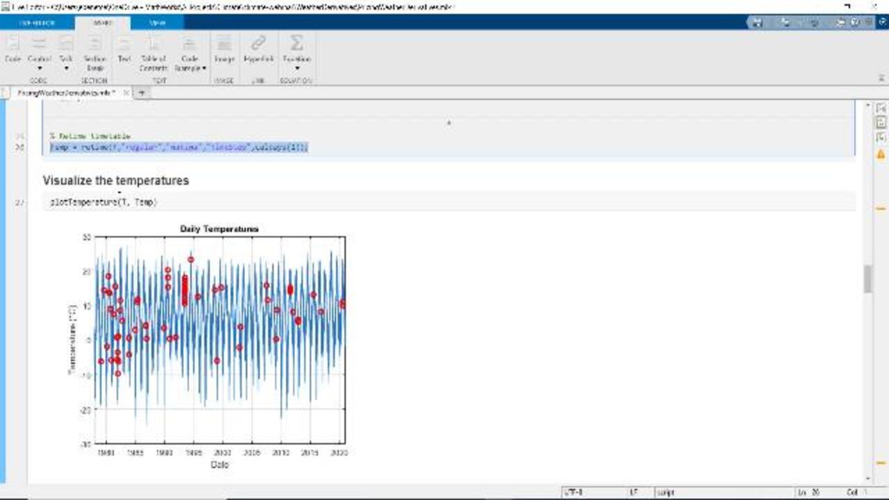
So the first thing I'm going to do is, I'm going to use a utility that you have in MATLAB called a Live Task, where you can actually easily interpolate the data within a timetable. Now, to insert this little app within my own script, I went to "Insert," "Tasks," and then selected "Retime Timetable." And you see that there's other utilities, all that work with timetable data.
Now, this little app or little utility will allow me to interpolate timetable T, using a single day, "Time Step," and then using a cubic interpolation for the rule. But there's a few others that you could have selected. And the advantage of these apps is that, as you make changes to the app, the app will, in the background, build the necessary code or the equivalent code for this process so that you don't have to remember the syntax or even call it yourself.
And then at the end, I have a little utility that just plots the temperature that has been cleaned. And you'll see that on the blue, there's the temperature I collected. And the red dots are the dates that I had to interpolate to actually get a complete data set.
Once I have the temperature, the next step is to actually model this temperature such that I can forecast some values into the future. For this, I'm going to use a process that's very similar to an econometric modeling. First of all, I'm going to remove the seasonality in data, if any, and then I'm going to use an ARIMA model to model the volatility within it.
So how we determine this is not in the data? So first of all, I'm going to use the detrend function on MATLAB to remove the linear trend within it, if any. And then I'm going to use the signal-processing function, called periodogram, to check the frequencies.
Now, when I look at the spectrum, you see that, as expected, the top periods are a full year, 365 days. And there's a half-year period of 182. And this is quite normal in this type of data. The temperature is periodic within a year, as it's colder in the winter and it's hotter in the summer.
So based on this analysis on the spectrum of the signal, I'm going to build a linear model, so just follow. And the paper that we referenced at the beginning of this talk, you'll see that they used a very similar model for it. Just for completeness, this would be the paper that I'm referring to here.
Now, going back to the model. So how do you fit such a model in MATLAB? These are your models, since you can see that all the coefficients, A, B, C, D, and E, are multiplying the independent variables. And therefore, I can just use the fit linear model function with my temperature model and the temperature data I have.
And this could be the equivalent command. We have the time, again, in time difference, my designMatrix, which is basically the coefficient of this function, and then the model. So once I run this, you'll get the fitted model.
Now, one of the most interesting things that you'll see on this model is that the linear term, or just B, is not zero. And it's actually a very clear or a very relevant term, with other value of 0.38. Now, the way to interpret this value is that the temperature at this location is increasing at a rate of 0.38 degrees per year, which is quite consistent with all temperature models saying how much the Earth is going to heat during this year. If you want to see this trend, it's very clear that if we fit our deterministic trend and we plot this linear value, we clearly see the increase in temperature over the last 40 years.
Now, once we have this trend correctly fitted, the next step is fitting the volatility of this model. Now, if you go to the original paper, you'll see that this process is done a bit differently. But in this case, we're going to simply use a ARIMA model within MATLAB, ARIMA/GARCH .
And in here, we'll be, first of all, using the residual trend. We're going to get the residuals. And we're going to use the function, arima, to fit this ARIMA/GARCH model. And you'll see that the autoref is Lags, and the minority Lags are all-- you can check that those are pretty good fits. But for the purpose of this example, you're going to leave it as those. And you see here the actual result of the model.
So finally, once we already have the deterministic trend of the temperature fitted and we have the volatility model, using an ARIMA model, simulating future temperature scenarios is quite straightforward. And we only need to fit these two models the actual values over the next years. So in this case, I'm going to model the next two years, so 730 days. And then I'm going to predict the deterministic trend, using my linear model. And then I'm going to simulate my volatility, using the ARIMA/GARCH model, and I'm going to do it for a total of a thousand different paths. This is the Monte Carlo approach to the problem.
The total value of the temperature is going to be the sum of the two. And when we want to visualize it, as expected, we'll see that there, we get the plot of different trends for the next two years. So the little colors in the background would be the Monte Carlo paths of our temperature.
The middle yellow line could be the mean temperature, or the median of these paths. And the two yellow lines would be the confidence interval. The green line, or the green path, is the actual temperature that we observed during 2021. And you can see that our model predicts very well where these temperatures are going to be.
So finally, once we have the temperature model, then you can see that the model is quite good, at least for the upcoming years. Pricing the derivative is quite straightforward. We simply need to plot this temperature, this forecasted temperature, into the pricing function. Remember that is based on the accumulation of heating degree days, the finest days where we deviate from 18 degrees.
So this is a simple formula, and you can see how this produces a very nice histogram on the probability of this base happening on all the different paths that we simulated. And of course, by defining a strength level and a price-tag number, we can simply get a histogram of the price of the option. And of course, as the strength increases, you can see that the bucket around zero does the same.
So finally, just to summarize the whole example and the steps that we do to get here, first of all, we first use the functions, webread and webwrite, to get the temperature data from a REST API. We then process the timetable data, using the function, retime, to interpret missing values, and then periodogram to analyze the spectrum and get the 365-day cycle. After that, you use the functions, fit linear model and arima, to fit the deterministic trend as a linear model, and arima to fit the volatility of the temperature. And finally, once we had this model, we used a histogram to plot the distribution of prices of weather derivatives across the next two years.
Featured Product
MATLAB
Up Next:


Related Videos:


Select a Web Site
Choose a web site to get translated content where available and see local events and offers. Based on your location, we recommend that you select: United States.
You can also select a web site from the following list
Americas
- América Latina (Español)
- Canada (English)
- United States (English)
Europe
- Belgium (English)
- Denmark (English)
- Deutschland (Deutsch)
- España (Español)
- Finland (English)
- France (Français)
- Ireland (English)
- Italia (Italiano)
- Luxembourg (English)
- Netherlands (English)
- Norway (English)
- Österreich (Deutsch)
- Portugal (English)
- Sweden (English)
- Switzerland
- United Kingdom (English)