Reduced Order Modeling with AI: Accelerating Simulink Analysis and Design

[MUSIC PLAYING]

Welcome to MATLAB EXPO's Reduced Order Model with AI-- Accelerating Simulink Analysis and Design.

My name is Terri Xiao. I have been with MathWorks for nearly 15 years. And my background is in control and dynamics.

Hello. My name is Kishen Mahadevan. I'm a product manager with the Controls Marketing Group at MathWorks. I've been with MathWorks for close to five years now. And I have a background in controls and dynamics as well.

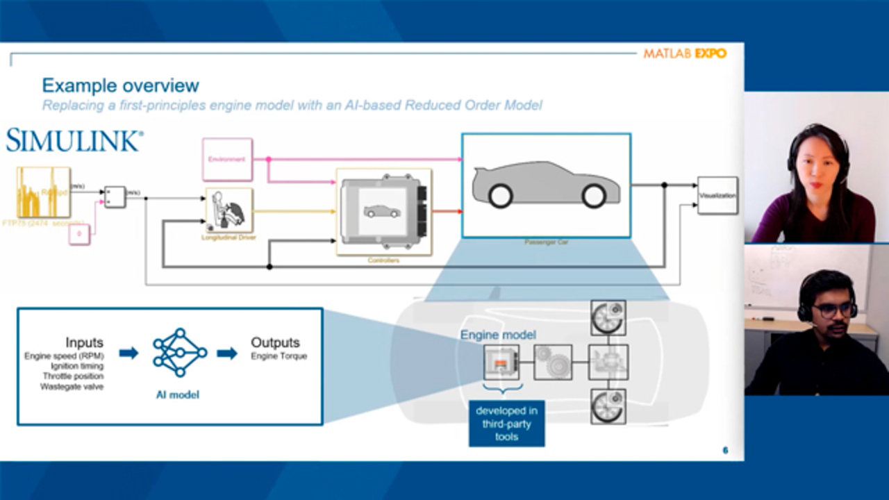
Great. Thank you. So let's dive in. We will be using the Simulink model throughout the presentation. So let's get familiar with it. This is a passenger car model. The model consists of a controller, car engine, visualization, et cetera. The car engine model is from a high fidelity third party tool. Let's run the model.

Well, as you can see, this is running relatively slow. But I can assure you that I have tried everything, like picking a [INAUDIBLE], removing all edge break loops, setting the right initial state, et cetera. How am I going to run this model in real time or run it for hundreds of times to check for test cases scenario?

Terri, have you heard of reduced order modeling?

Do you mean like a table lookup?

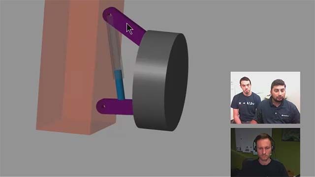
It could be. But where do you start a modeling is more than that. Its original modeling is a set of techniques that help you reduce the complexity of your model, while providing reduced but acceptable fragility. So let me actually show you a video of this model running in hardware-in-the-loop.

The only change I'd make is that I use a reduced order model to replace the high fidelity model component that you showed. And now, because of that replacement, the simulation runs much faster, thereby enabling hardware-in-the-loop testing.

And the video that you see on your screen now shows the reference signal, as well as the prediction from the AI model running real time on a Speedgoat machine.

So throughout this presentation, we will show you how we got here. That is, by diving deeper into what is ROM, why use ROM, how to create one, and how to integrate that into your system.

Great. So it sounds like, at the end of the presentation, you should walk away knowing that you can enable hardware-in-the-loop testing and system-level simulation for high fidelity model. And you can also explore various reduced order model techniques in MATLAB to find the best method for your specific application.

So before we get into solution mode, let's talk about the common challenge control engineers face. So for the purpose of this presentation, I am assuming the role of a control engineer, while Kishen, my AI expert, will dive deeper into the detail on reduced order model creation.

So one common challenge that we heard is that you are given a high fidelity model from the Component Designer Group and you need to perform hardware-in-the-loop testing with the model, but can you run such a high fidelity model in real time?

Next, you realize you need to make the model run faster, but there is a wide range of methods available. So how do you create a role model that balance the result of good speed, accuracy, and interpretability? So let's see how MATLAB can help address these common challenges.

Before we jump into how to create reduced order models and how it helps solve those challenges, I want to get us all on the same page and talk about what is reduced order modeling. So reduced order modeling is a set of techniques for reducing the computational complexity of a computer model while providing reduced but acceptable fragility.

Now, why are these techniques important, and what are some of the use cases? There could be several reasons why somebody might want to try reduced order modeling. One could be to enable system-level simulation by bringing reduced third party FEA models into Simulink. The second use case could be like the challenge we have in hand-- to perform hardware-in-the-loop testing. That is, by reducing the high fidelity model, you may now enable it to run in real time for hardware-in-the-loop testing that was not really possible before.

And another use case could be to develop, say, virtual sensors or digital twins. Say for the virtual sensor use case, you can create virtual sensors from data, when the signal you want to measure is not directly measurable or when the sensor is too expensive. Or for the digital twin case, you may want to create a reduced order model of a real hardware to serve as a digital twin.

And another use case we've seen is to perform control design. For example, with nonlinear model predictive controllers, where there is a need for fast nonlinear prediction models that can be used in real time to solve an optimization problem.

And finally, it could just be used to run hundreds or thousands of desktop simulations. And you may need to run so many simulations either to optimize design parameters in your model or for test requirements, or check for all the corner cases. So let's talk a little bit about the "how" next.

You can use AI-based or data-driven techniques to create reduced order models, where you collect input/output data from a high fidelity first principles model, and then use that data to train an AI model using machine learning, deep learning, or system identification techniques.

Now, one question that might come up is, are AI-based techniques the only options to create reduced order models? The answer is no. There are other techniques in which you can develop reduced order models. And MathWorks provides tools for those methods as well. And these techniques include linearization-based reduced order models as well as the model-based reduced order models.

So if you're interested in learning more about those techniques, please reach out to us and we'll be more than happy to talk to you about them. But the focus of today's session is going to be on AI-based reduced order modeling. And more specifically, we're going to look at how you can create an AI-based ROM that can replace the original high fidelity engine model that Terri briefly introduced before with an AI-based reduced order model.

And one thing to note here is that this AI model that we will end up creating will coexist with other components in your Simulink model, which can be created using first principles. So let's jump into creating this AI-based model.

And the standard workflow that we'll follow to create any AI-based model is that we start with the data preparation step. We then jump into AI modeling, where we use the data that we collected to model our AI system. We'll then bring that trained AI model into Simulink for system-level simulation and testing, and, finally, generate code for deployment.

The first step here is data preparation. And this step involves collecting data from the system. So Terri, considering that you know more about the right set of signals to vary to capture, say, the right dynamics for the engine model that we have at hand in your Simulink model, could you please help with the data preparation step?

Sure. So in this case, you need to generate enough data from simulation to create a good reduced order model. But running high fidelity simulation is expensive. So the challenge is, how do you do design of experiment to generate sufficient amount of data, but at the same time not run too many expensive simulations of a high fidelity model?

So first, we need to pick the model parameter we want to vary and their range. So for example, we are changing, in this case, the engine torque, the command, and ignition timing here. We create a design of the experiment table with all the possible combinations of parameters. So in the Simulink model, we have a design of Experiment Manager that varies the value of this parameter with every experiment. And then we lock the data and run it.

So after we run all the combinations of the simulation, then we can just go in and use those data as needed.

That's perfect. So we now have the data that we can use for AI modeling. That's great. That brings us to the next step in the workflow, which is AI modeling.

So now, again, here, there are a lot of different AI techniques that are available. But if you were to specifically look for, say, AI techniques that work well for modeling dynamic systems, these are the popular ones. And these are the ones that will most likely show up. And these techniques include deep learning methods, such as neural state space or Neural ODE, LSTM, or Long Short-Term Memory networks, or even system identification techniques such as nonlinear ARX models.

In the interest of time, I will not be able to go through each of these techniques in detail. But I will go through the neural state space to give you an idea of how you can model that in MATLAB, and then briefly introduce LSTM, as well as the nonlinear ARX models, before I circle back and compare and contrast and mention a few advantages of these techniques over another.

So let's start with the neural state space technique. So the basic concept behind the neural state space model is that it is in a familiar state space form, where the nonlinear state function f and the nonlinear output function g in the nonlinear state equations will now be in neural networks-- that's the image that you see-- that you will learn from data. And this is also popularly known as neural ODE within the deep learning community.

Let's now take a look at how you can model such a system in MATLAB. So the first step is we start by loading the data that we generated synthetically. That is the data that Terri passed on to us. We then prepare the data for training. This includes data processing steps, such as downsampling, which could help for the training, normalizing, and splitting the data into training and validation sets. And the plot that you see on your screen shows the training and the validation data for our four inputs and one output.

The ones that you see in blue are the split between the training data, and the one in orange is the validation data set. And once we have the data ready, the next step is defining and training the neural state space model. The first step is to define the neural state space model. In our case, we have one state, which is the engine torque that we want to model, and then four inputs. Once we have that set up, we then configure the state network.

In our case, the output is equal to the state, which is the engine torque. So we're not learning a separate output network. We then specify the training options, and then train using the nonlinear state space estimation command.

And as you can see, with the nonlinear state space estimation API, we have made it easier for controls and simulation engineers, who might not be experts with deep learning to still leverage such API techniques and create these models. And once we have this model trained-- here, I'm loading a pre-trained model-- once you have that trained, you can validate this model with the independent data set that we initially split.

And on looking at the results, we see that the reduced order model, which is our neural state space model in this case, is able to match the simulation results from the high fidelity model for the same input data. So this is a great candidate to be used as a reduced order model now.

An alternate approach to neural state space is to create the Long Short-Term memory network, or LSTM network. And this network is nothing but a type of a recurrent neural network that can learn long-term dependencies between time sets of data. And that's why it's also a good technique to use for dynamic systems.

And to create such a network, you can either use command line functionalities or use an interactive app, such as the Deep Network Designer, that helps you create and train these models without writing any complicated code. In this case, that's what I used. I use the Deep Network Designer app at my end to create and train this network. And that's the image that you see on the screen.

And the last approach that I tried out at my end and that I want to specifically call out is the nonlinear ARX models. And the reason I want to talk about this model is because it's unique in a way, where you have the flexibility to choose regressors to be physically meaningful signals, like saturation. Or you can also start by estimating linear models, and then use any of the nonlinear function estimators on top of it, which include machine learning techniques as well, to capture nonlinearities in the system.

So you have the flexibility to include your physical insights here with this model. And the configuration that I selected with nonlinear ARX at my end is to try for this reduced order modeling case at hand was I chose a set of linear regressions and I leveraged the machine learning algorithm of Support Vector Machine to create the reduced order model here.

So as we went through briefly across these multiple techniques, we saw that there were many hyperparameters that you could choose from for training. In such situations, you can leverage Experiment Manager to design and run experiments to identify the best configuration for training your AI model. And just to give you an idea, the experiment that you see on the screen here was when I created a script that changes the layer size for the neural state space model.

So I varied the layer size from a very low value to a high value, and I ran an experiment to see which of those gives me the right set of metrics and the accuracy that I'm looking for. So this is one way you can go about trying out different sets of hyperparameters and figuring out which one works the best for your use case.

But this setup in itself can be extended to run experiments for other techniques that we briefly spoke about, and can eventually be used to compare different AI models and techniques in itself.

So looking back at all the AI models we've trained, one thing I want to point out before I talk about the table that you see on the screen is that choosing one particular AI model is not always about, say, accuracy or one metric. It's a combination. And there may be other factors that you need to take into account, including training speed or deployment efficiency-- such as inference speed or model size.

And having run through these techniques and having evaluated those at my end, I have a table that summarizes results across these techniques across these metrics.

Terri, based on the initial objectives and the challenges that you mentioned, which of these models or metrics are more important to you, and which one would work best for your use case?

Well, since the objective is to run the system-level simulation at scale to test for all requirements and check on the cases, as well as performing hardware-in-the-loop testing, the inference speed model size matters here. However, we also have strict accuracy requirements. So the neural state space seems to be a good option.

So as you can see, with the pros and con comparisons here, we can see how MATLAB can address the common challenge and help make an informed decision when creating a reduced order model that can produce desired results.

That's great, Terri. It seems like a neutral state space model is a perfect fit. I'm now curious to see how this works well with your overall system.

Let's bring it into the overall system. So now that we have chosen neural state space, the next step is to integrate the trained model into Simulink. So existing Simulink blocks include machine learning and deep learning models-- so making bringing AI model into Simulink really simple.

So now that the engine component is replaced by a reduced order neural state space component for the system-level simulation, it runs much faster. And we can run hundreds of simulations checking all requirement and corner cases to ensure that the AI model performs as expected.

So next, we we will see how we can deploy this deep learning model to a Speedgoat machine for HIL testing. Hardware-in-the-loop serves as the last functional test of the designed component before we move into final system integration. So in hardware-in-the-loop, we are generating code for the component we are designing and for the plan model as well.

The plan model in this case includes the train-your-own state space AI model that runs on the real-time computer, while the controller runs on the target platform. So Simulink can be used to monitor signal and address parameters on the deploy model.

Here's a quick demo showing HIL testing. So we are seeing the reference signal and the prediction from the AI model running in real time in this Speedgoat machine. We have shown you that, using ROM, control engineers can address the common challenge of a high fidelity model running to slow or it can't perform HIL testing.

So another form of deployment is to use any of our cogeneration tool to deploy model from MATLAB or Simulink to any target. This can include generating library-free C code or code with Optimization Library for AI model to target specific hardware.

On top of deployment through hardware-in-the-loop or cogeneration, we can also use ROM outside of Simulink for development and operation stage. So we have seen a deployment to Speedgoat hardware. And through the use of Simulink compiler, we can exploit a plan model as the FMU for integration to third party tools.

And if you have a trained deep learning algorithm, you can also export it through the ONNX model format for interoperability with other deep learning framework. As we have mentioned previously, you can generate code for target-specific hardware.

Lastly, you can use MATLAB and Simulink compiler to create a standalone application for your digital twin need.

So here is an example from Renault, who is working on developing the next-generation technology for zero emission vehicle. So in this case, they're using deep learning technique to estimate the nitrogen oxide emission from the car. Even though not AI expert, Renault engineer predict nitrogen oxide emissions with close to 90% accuracy. And they were able to generate code directly from the network for ECU deployment.

Well, we're at the end of the presentation and we really want you to walk away knowing that you can enable HIL testing and system-level simulation for a high fidelity model with ROM. And you can also explore various ROM technique in MATLAB to find the best method for your specific application.

Thank you very much for your time.

Thank you, all.

[MUSIC PLAYING]