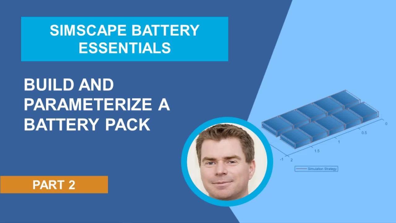
Build and Parameterize a Battery Pack | Simscape Battery Essentials, Part 2
From the series: Simscape Battery Essentials
Simscape Battery™, a new product in R2022b, has been developed to provide a technology development framework that is assembled specifically to create a bridge between battery cell and battery system. The bridge directly supports upskilling as well as design exploration and design rigor, meaning you can navigate the battery system technology development cycle rapidly and with confidence. You will learn how to:
- Define the components and geometry of a battery pack.
- Make the battery pack parameters available in a MATLAB script.
- Visualize the pack geometry.
- Automatically build the battery pack in Simscape.
- Simulate the battery pack in a simple test harness.
Published: 20 Sep 2022
Hello, everyone. My name is Graham Dudgeon. And welcome to part 2 in a series of videos where we'll provide insights and work examples on the use of Simscape battery, a new product in the Simscape portfolio. Simscape battery has been developed to provide a technology development framework that's assembled specifically to create a bridge between cell and system. The bridge directly supports upskilling as well as design exploration and design rigor, meaning you can navigate the technology development cycle rapidly and with confidence.
Today, I will show you how to build and parameterize a battery pack. I'm going to be working from one of the shipping examples you can find in the documentation. Build a simple model of a battery pack in MATLAB and Simscape. So what we have here is the MATLAB live script, which has the complete workflow.
Now, in part 1, we worked up to the module level. So we take a look at this visual here, the steps that we take to go from cell to pack. We go from cell to parallel assembly to module. Now, those were the steps we took in part one. Today, we're going to move from the module to the module assembly to the pack.
And so what I've already done is I've run the lines of code to create the module for this specific example. What I'd like to do before we take the next steps is just show you the visualizations of the cell, the parallel assembly, and the module for this specific example.
So we're using poached geometry in this case. So the best way to show you that is to show you the image. And so let me just put battery cell for our image using the battery chart function. And so here you can see the pouch. And notice that the tab location is opposed. So you can see the tabs on either side here.
Now let us look at the battery parallel assembly. So what we're doing is we're connecting three of the cells in parallel. So just refresh battery image with the battery parallel assembly. So here we see our parallel assembly.
Now, if I actually just quickly take a look at our parallel assembly object, our model resolution is currently set to lumped. So if I go to our image and see show simulation strategy, you can see there is a single boundary around our parallel assembly indicating that the parallel assembly will be modeled as one cell with this setting. For more information on how to change the model resolution, please refer to part 1 in this series.
So let's move on up to our module. Now, with the module, we are connecting 11 parallel assemblies in series. Let's just visualize that. Change our image to battery module. And I'll show you the simulation strategy. So we now have a single boundary around our battery module. And if we just take a look, we've set the model resolution to lumped.
OK. So now what we're going to do is we're going to take the next steps to build up to the pack. So we have our module. Next step is to create a module assembly. So we use the module assembly function. So let me just highlight and evaluate this code. And you can see here that we've defined an intermodule gap of 0.1 meters. And we've also said create a module assembly that consists of two battery modules.
So let us visualize this. So here is our module assembly. And if we look at our simulation strategy, remember we defined our module as lumped module resolution. Our module assembly will be modeled as two individual cell models when we are ready to create this Simscape model of the system. And you can see the intermodule gap, 0.1 meters in this case.
If we just take a look at the battery module assembly object, we can see that we have connected those two modules in series. Recall that the electrical connections that we are specifying are independent of the geometry. So series connection, we connect plus to minus. Parallel connection, we connect plus to plus, minus to minus. And that is independent of the geometry.
I'll also just call out two object properties that we have with our module assembly. One is the packaging volume. So as we're building our battery pack up, Simscape battery is keeping tabs on the overall volume as we build up. We can also look at the cumulative mass. And so we're currently at 6.6 kilograms for this battery module assembly.
Let's now create the pack object. What we're doing here-- I'll just highlight and evaluate. We are connecting five module assemblies. And if we look at all properties, the circuit connection is a series connection.
Let's visualize this. Change the battery pack. So here is our full battery pack. Module assembly consists of two modules. And then we have five module assemblies to create the pack.
If you look at simulation strategy, you can see that each module is defined as lumped. Each module will be modeled as an individual cell model appropriately scaled. So our pack will be modeled as 10 individual cell models. So we can take a look. Visually, we saw that we're going to have 10 individual cells. But we can just evaluate the number of models. And we see 10.
OK. Now what we're going to do is we're going to build the battery. Now, we see the line of code here. As it stands, we see we use the build battery function to use the battery pack and create a library called pack library.
I'm going to make a slight modification here. What I'm going to tell the build battery function to do is to set initial targets and parameters as variable names. What this is going to do is it's going to create a MATLAB script which will contain the parameterization so that we can readily update and change the parameterization from a MATLAB script. So let's just create this. And then I'll show you the various elements. I'm just going to show the folder to show you the build process as it goes on.
OK. We have generated our library and also the parameterization script. So let's take a look at the pack library. So here we have our pack model. As you can see, we have various measured signals available. Module assemblies, we can take a look at the module assembly under there.
And if I just bring up also the library contains the elements that build up the pack. So we have the modules and the parallel assemblies in here. So we have access to each stage of the build. It's all available to us.
So if I double click on the pack-- let me just expand this out. Actually full screen. Space bar. So you can see here that we have our five module assemblies all suitably instrumented. Double click now on module assembly 1. And we have our two modules suitably instrumented.
If I now click on module 1, you will see that we have a data structure called module type 1, which contains the parameterization. You may remember in part 1, if we do the default build, it will put numerical values in here. When we specify we want to create a parameter file, then we have access to these data structures. So let's close this down. And let's take a look at the parameterization file.
So when the parameterization file is created, it uses default parameters. But you can, of course, change those to your specific data sheet values. And you can see that we have access to parameterization for module assembly 1 module 1, assembly 1 module 2, et cetera. We're going to stick with the default values for now. And we'll change them as we move forward.
What we'll do now is put this pack in a simple test harness. And we'll discuss some aspects of the simulation. So let's just click and drag the pack across. I just want to connect this to a resistor, so a very simple test harness. Do Control-R to rotate the resistor. Connect it up to the terminals. Just double click on the resistor. We see if resistance is 1 ohm, I'm just going to leave it as that.
I also want to add an electrical reference and a silver configuration block. I'm going to set the solver configuration to use the local solver with a sample time of 0.01.
OK. We have access to various measurements within the pack. What I'm going to do is I'm going to look at state of charge and also voltage of the cells. So let's set this up. I'm just going to terminate the signals. I'll do the state of charge and also cell voltage.
I'm going to just click on the three dots and see a log selected signal. By logging the selected signals, they will be made available within the simulation data inspector. I'm just going to terminate the other signals for the sake of tidiness.
One more thing we need to do before we run is run the parameterization file. I'll just open this up. And we'll just run it. OK. We are ready to simulate the battery pack.
Let's take a look at the data inspector. So we have state of charge and also cell voltage. If I just click, it's going to ask me what I want to do with these multidimensional signals. So you convert the channels so you get access to each one individually.
So let's take a look at state of charge. So default, 100% state of charge for each module. So they're all the same at the moment. Cell voltage, just over 35 volts for each module. And they're all equal as well.
So what we want to do now actually is let's change the parameterization to change the initial state of charge for some of those modules. So let's go back into our parameterization file. Let's focus on assembly 1, so module 1 and module 2. So we see we have the state of charge definition here. Let's just change it to see 0.4 for module 1, 0.6 for module 2. Just save that and run it. Go back to our simulation, run our simulation.
Now let's take a look. We just convert these to individual channels. Take a look at state of charge. State of charge 1 starts at 0.4, 2 starts at 0.6, and the rest are still defined as 1. So you can see how we can change that parameterization within the MATLAB script and have it readily available to the simulation model.
So to recap, what we've looked at in this session, we have went from a module definition to a module assembly and from a module assembly to a pack. We have shown how to build the pack model using the build battery function and how to add parameterization in a MATLAB script so we can readily access the parameters and change the parameters for the simulation. I hope you have found this information useful. Thank you for listening.
Related Products
Learn More


Select a Web Site
Choose a web site to get translated content where available and see local events and offers. Based on your location, we recommend that you select: United States.
You can also select a web site from the following list
Americas
- América Latina (Español)
- Canada (English)
- United States (English)
Europe
- Belgium (English)
- Denmark (English)
- Deutschland (Deutsch)
- España (Español)
- Finland (English)
- France (Français)
- Ireland (English)
- Italia (Italiano)
- Luxembourg (English)
- Netherlands (English)
- Norway (English)
- Österreich (Deutsch)
- Portugal (English)
- Sweden (English)
- Switzerland
- United Kingdom (English)