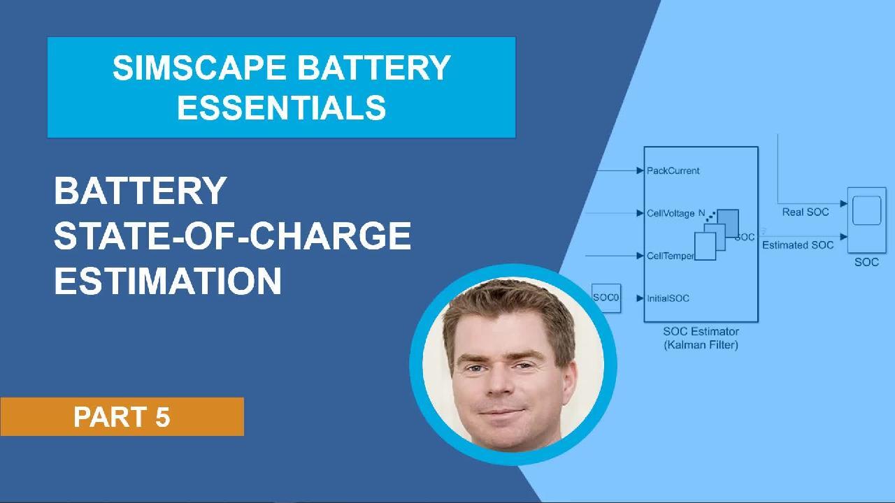
Battery State-of-Charge Estimation | Simscape Battery Essentials, Part 5
From the series: Simscape Battery Essentials
Simscape Battery™, a new product in R2022b, has been developed to provide a technology development framework that is assembled specifically to create a bridge between battery cell and battery system. The bridge directly supports upskilling as well as design exploration and design rigor, meaning you can navigate the battery system technology development cycle rapidly and with confidence. You will learn how to:
- Connect a battery cell with a Kalman filter state-of-charge estimator.
- Simulate different Kalman filter types for a given charge-discharge cycle.
- Compare the state-of-charge estimations using the Simulation Data Inspector.
Published: 20 Sep 2022
Hello, everyone. My name is Graham Dudgeon, and welcome to part 5 in a series of videos where we will provide insights and work examples on the use of Simscape Battery, a new product in the Simscape portfolio. Simscape Battery's been developed to provide a technology development framework.
This is sampled specifically to create a bridge between cell and system. This bridge directly supports upskilling as well as design exploration and design rigor, meaning you can navigate the technology development cycle rapidly and with confidence. Today, I'll show you how to estimate state of charge of a battery using a Kalman filter.
The example we're working from today is battery state of charge estimation, which you can find in the documentation. First thing I'll do is open the MATLAB script. You see, there are three lines of code in the script. So if I were to run this code as is, what would happen? It will open the model, set the parameters appropriately, simulate the model, and then show a response.
I go back to the documentation, it will provide this state of charge plot within MATLAB. I'm not going to do that today. I'm actually going to delve a little bit deeper into the simulation model itself. We'll explore the model, and we'll also talk about certain modeling characteristics and why we've included them in this example.
So all I'm going to do is open the system. I'm just selecting that line. Right click. Evaluate Selection in Command Window. And this will open the model. OK. Here's the model. So let me just expand that to full screen. Press Spacebar. First thing I'm going to do is actually just simulate this. So we'll run it.
I'll show you the result in the simulation data inspector. We've actually got two options here. You can see the results in the scope block. I'll just bring this scope block over so you can see that. Expand to full screen. So real SOC is our simulated state of charge.
As we're running a simulation, we have the benefit of being able to calculate state of charge directly. From a practical perspective, we cannot directly measure state of charge. So we need some form of estimation to be able to do so. But you can see here that our estimated state of charge starts at a different initial state of charge but then very quickly converges onto the trajectory of that measured state of charge and then tracks it quite well.
You'll see that is noise here, and we'll talk a little bit more about that as I dig a little bit deeper into the example. Let me close this down. I can also view simulation results in the simulation data inspector. So the way that we make those signals available to the simulation data inspector.
So I go to a signal here. Notice the little Wi-Fi symbol. If I click on the line-- see the three dots appear? I hover over that and go here. And it says Stop Logging Signal right now because I've already selected that. But this is a selection you would make to start logging the signal.
Also on the measured state of charge, same thing. So we have these two Wi-Fi symbols, meaning real SOC and estimated SOC are available within the simulation data inspector. So let's take a look at that. And I'll just click. Realize we'll see an estimated SOC. You can see we have the same plot as we saw on the scope.
Now, why would we use a simulation data inspector rather than the scope? Well, today, I'm going to be running multiple simulations. I'm actually going to change settings within the Kalman filter, and I want to directly compare one simulation run against the other. And so the simulation data inspector is a good environment for me to do that.
So let's go to the model, and we'll talk about some of the components that we have in this model. First of all, we have a table-based battery block. I just double click there to open up the block parameters. So we have characterized this battery using state of charge, temperature, voltage, and resistance vectors and matrices and cell capacity.
Let's just take a look at the data in the MATLAB workspace. OK. So if I look at the state of charge vector-- so you see it was categorized state of charge with seven data points. Temperature vector. In this case, three data points. These temperatures are in Kelvin. Open circuit voltage is a matrix.
Each column relates to a temperature and the temperature vector, and the rows relate to the state of charge. So there are seven rows. You can also look at terminal resistance and finally capacity. The point I'd like to make here is these matrices are quite small for the purposes of demonstration, but you can characterize these table-based models to whatever level of granularity you want.
Final point. If I go down to Thermal. See thermal port, it's set as model. So we have a thermal port exposed here. That's the orange line. If I was to set that to omit, it would remove that thermal port. I'm going to leave it as a model. On the thermal side, we have a controlled temperature source, 292.15 Kelvin.
We're measuring temperature with a temperature sensor. That measurement of temperature is going into our Kalman filter. We are also measuring voltage across the cell. That also is going into our Kalman filter, but we are introducing sensor noise to emulate real world effects.
In terms of the current, what we have is a current profile here. I'll just double click on this. It's taking measured state of charges and input. I won't dwell on this, but what it's doing-- when charging, it will charge at a constant rate of 15 amps. But when discharging, we are introducing some variability with white noise and with uniform random numbers in order to provide the discharge with some variability so that we can better test the accuracy of the estimation.
We feed the current profile directly into a controlled current source to drive that battery. And as a measurement, we take it, add some sensor noise, and put that current into our Kalman filter. So let me show you what the state of charge estimator is in the Simscape Battery library. We go to Simscape. Battery. BMS. Estimators.
And the estimator that we're focusing on today is the Kalman filter state of charge estimates. You can see that we also have an adaptive Kalman filter and Coulomb counting for charge estimation, and also a state of health estimator, which is based on degradation and resistance. I'll now double click on the estimator.
So we have four choices for the filter type, extended Kalman filter, extended Kalman-Bucy, unscented Kalman, and unscented Kalman-Bucy. The key point I'd like to make with these estimators. While there are additional parameters that you can set, the key point is you need a system model. And you can see that I'm using the data that parameterizes the battery table-based block.
So we just ran the extended Kalman filter. Let me select extended Kalman-Bucy. Apply. And we'll now run this. And now we look at the data inspector. I have accessed run 1 with the extended Kalman. Run 2's the extended Kalman-Bucy.
So let's just look at estimated start of charge with the extended Kalman. That's purple. It's changed the estimation for the Kalman-Bucy. Let's change it to purple. Let's just zoom in on the discharged profile. So you can see we have some differences in the estimation, which is a consequence, of course, that we're using different estimation algorithms.
Let me just quickly go through the unscented. Simulate that.
And we'll do the unscented Kalman-Bucy as well. Simulate that.
OK. Let's take a look at our simulation data inspector. I will select the estimations for our other simulations. Just changing the colors as I go. Let's look at our charge profile here.
So you can see we have different results. We're using different estimation algorithms. So if I was doing a more thorough investigation of this, I would look at relative error of these estimations, and I would also configure these simulations to cover up a much broader design exploration space. So we changed the white noise profiles, we changed charge discharge cycles, but that can all be readily done within the simulation framework.
So to recap of what we've looked at today. We have looked at battery state of charge estimation, specifically using the Kalman filter book within Simscape Battery. And we can see from this model we have both thermal and electrical effects. We use the table-based battery block in order to parameterize the battery, and that table data was also used to provide model information for our Kalman filter.
We added current and voltage sensor noise using white noise blocks in order to emulate real world measurement effect. I hope you have found this information useful. Thank you for listening.
Related Products
Learn More


Select a Web Site
Choose a web site to get translated content where available and see local events and offers. Based on your location, we recommend that you select: United States.
You can also select a web site from the following list
Americas
- América Latina (Español)
- Canada (English)
- United States (English)
Europe
- Belgium (English)
- Denmark (English)
- Deutschland (Deutsch)
- España (Español)
- Finland (English)
- France (Français)
- Ireland (English)
- Italia (Italiano)
- Luxembourg (English)
- Netherlands (English)
- Norway (English)
- Österreich (Deutsch)
- Portugal (English)
- Sweden (English)
- Switzerland
- United Kingdom (English)