Vehicle Powertrain Modeling and Full Vehicle Simulation Using MATLAB and Simulink for Student Competitions
M V Krishna Teja, JK Tyres
Overview
In this webinar, we will provide an overview of how to use MATLAB and Simulink for powertrain modeling relevant to student automotive competitions and projects. First, you will learn about powertrain modeling and how to actuate vehicle models with power sources, build driveline mechanisms, model batteries, and model engines using Simscape and Powertrain Blockset. Then, our guest speaker M V Krishna Teja, will demonstrate a full vehicle model with its subsystems suspension, powertrain, brakes, tires, simple control systems and run it on a racetrack.
Highlights
- Thermal management system
- Electric vehicle powertrain
- Full vehicle simulation on a race track
Guest Speaker
M V Krishna Teja
M V Krishna Teja joined JK Tyres in 2021 as scientist. Working at Raghupati Singhania Centre of Excellence (RPSCOE) - one of India's leading industry-academia collaboration between Indian Institute of Technology Madras and JK Tyres, his research primarily focuses on driver-vehicle-tire interaction using SiL/DiL simulators, tire tuning, ADAS and autonomous vehicles. Before joining as a scientist, he was pursuing PhD from the same lab, RPSCOE IIT Madras in the field of vehicle dynamics control and reinforcement learning.
Recorded: 3 Nov 2021
Hi, everyone. This is Veer from the MathWorks Student Competition team. And welcome you all to the second session of the Vehicle Design Webinar Series for student competitions. So today we'll be talking about vehicle powertrain modeling. We'll touch base on that. And then we have Krishna Teja from JK Tyres. So he'll be talking about full vehicle simulation. And he has a lot of content to share with you. So you have to be with me for some time.
And along with me, I have Sudhakar, Pratyay, and Himanshu who will be supporting the event. Now just a few recap things for the webinar. So this is the CDs which we are doing this October and the month of November. So first one we conducted on vehicle dynamics focusing on vehicle dynamics simulation. So if you have not attended it, you won't be getting the links for the recordings.
However, we'll be publishing the recordings. So if you haven't, you can reach out to us at racinglounge@mathworks.com with the email saying that you want the recording. Or you can also join our Facebook group, the link to which we'll be sharing at the end. Then today we have this completely dedicated session on vehicle powertrain modeling and full vehicle simulation.
And then on 11th of November, where my colleague Sam will be presenting. So it will be beyond simulation. You'll touch base on how to communicate with CAN networks using vehicle network toolbox. So if you haven't, again, we have shared the link in the chat. You can register for the 11th November session as well. There you will be learning communicating with the CAN network using vehicle network toolbox.
Now there are a few quick important things before we deep-dive into the webinar. If you have any technical questions, please use the Q&A section. And make sure that you are sending to all the panelists. And then chat box, chat box we'll try to use it for interaction for interacting with each other. So we'll be asking some questions, only a few not a lot of questions. So you can answer that in the chat box.
And then if you have some non-technical things, for example that can you zoom in, zoom out? It's not audible. The video is not proper. That, you can mention that in the chat box. Certain questions coming up that you're not getting the emails. So we haven't sent the email yet for the last session. We are in the process to publish the recorded video for the last session. We will send you within five to six business days.
So you'll be getting that. Otherwise, if you're not getting that as mentioned, you can reach out to us at racinglounge@mathworks.com. Again, we'll share the contact details and the link to the Facebook group at the end of the session. OK. So in the last session, we covered this. We covered these topics, racing line optimization where we saw one of the submissions from-- Jacob submitted his project for MathWorks Excellence in Innovation Program.
And this was also an introduction to MATLAB. And we also share a lot of resources from where you can download the code. Then Sudhakar, my colleague, he spoke about the equation based vehicle modeling using Simulink, where he demonstrated how equations can be converted into a block diagram representation. Further, we use vehicle dynamics blockset to model longitudinal and lateral vehicle dynamics.
And we also saw how you can add one driver, which was a Stanley driver to track certain parts. And then finally, we also covered in detail the multibody suspension system, which is a part of Simscape vehicle template. And we also demonstrated that from 2021b, you can also add a tire model to your multibody vehicle model. So this all, again, if you have missed it, don't worry. We'll be sending all the resources. And you can reach out to us on racinglounge@mathworks.com for more.
So with this, we'll have some exciting agenda and a little bit tight agenda today. So we'll be focusing on physical system, modeling of physical system. The whole session, I would say 1 and 1/2 hour session will be approximately, I think, 50 minutes will be dedicated towards modeling of physical systems, wherein we'll see a very basic battery electric model with motor cooling which will be based on the fundamental blocks.
And then we'll a little bit improve, or you can say add more details to a model where we'll be seeing how electric vehicle can be powered by BLDC motor. And then in powertrain blockset, that is also one of the toolbox that we, we have multiple vehicle reference applications which you can use for your different design purpose. And that will check out one electric vehicle reference application.
And then we'll see how Simscape, which is you can see equation-based modeling and powertrain blockset which is a data-driven modeling, how you can integrate these two. And then Krishna will come with his full vehicle simulation. And he has a lot to speak and a lot to show, and also he has a very nice introduction of himself. And then we'll share some resources. And then we can take some questions.
So with this, as we mentioned that most of the part, we will be focusing on modeling physical systems. So let's bring one image in front of you. And a very, very easy question for all of you, what is this like from the image from the physical system layout what you see? What can you think of this? What is this? You can write your answer in the chat box.
You have one one minute model, OK. RC circuit, OK. Equivalent circuit? Equivalent circuit, it's a circuit. Yeah, that's correct actually in electrical terms. But in terms of application-wise, what do you think? Which part is it for an electric vehicle? Battery modeling, OK. OK. OK. Single-cell model. Yeah, that's a correct answer, I would say. Yeah.
OK, Krishna is also answering. Thanks, Krishna. Yeah, so this is a battery or single-cell model. Now, the idea behind just to putting a rough diagram of this RC equivalent circuit or battery model, one-cell model is that this is what the physical system looks like, or physical system layout when we say. Similarly, you can also make one layout for a DC motor.
So this is LC or battery equivalent circuit. And to model this physical system layout or physical systems, we have a very interesting and exciting amazing tool called Simscape, which enables you to model physical systems. And what are these physical systems? Systems like thermal system, electrical system, mechanical systems, something that you can see, you can feel you can touch, and defined by using laws of physics.
And the one important thing is that, I mean, you must be seeing a lot of text on the slide. But the most important thing is basically it is just mimicking the physical system layout on a simulation platform, which is Simscape. So consider a DC motor. Now if you have to make a physical system layout of this, it will be having certain physical components. What are those components? Those components are resistors, inductors, electromechanical converters. And then for the load, you'll be having certain inertias.
So now when you're modeling that in Simscape-- so Simscape provides a certain good amount of physical blocks, wherein all the equations have been written. And then these each connections, for example over here if you see, these resistors, inductors, electromechanical converters, inertia, these are already having a set of equations. And these are interacted by energy exchange. So even the physical signal, what you see, it is having certain meaning over here.
So as I said, it is just a replica or mimicking the physical system layout on a simulation platform. As an example, here is a DC motor where you can see these elements. These elements are already having the equations. You don't have to derive it from scratch. You can connect it the way you connect in a real environment. And what you can further do is, for example, we are giving you a lot of different physical blocks which are there in Simscape library.
And if you want to customize it, for that you can use Simscape language. For example over here, you can see that we wanted a lossy ultra capacitor, a custom-made block. So for that, you can use Simscape language. And then what you can do-- so it's a long list, but in simple words since this is a webinar dedicated for powertrain modeling and basically full vehicle simulation, you can make an electric vehicle model. And you can perform optimization.
You can do component sizing and selection. And this is all code generatable if you're connecting it to the hardware or sending-- if you want the code to be done on a hardware. So important point from this is it is mimicking the physical system layout in a simulation platform which is Simscape. And then there's an energy transfer involved between these two components. Now once we say energy, this energy flow in this physical system, that is dependent upon across, and the true variable.
Now why are we telling this? Because this is helpful when you're making the connection. Because it might happen that if you want to send something like torque or maybe you want to send angular velocity, in that case how to do the connections. So across variables, I mean if you want to sense that, that is connected in parallel. And through, that is connected in series.
So here's one example in electrical terms. So power in electrical terms can be defined as voltage into current, where voltage is across, and current is a through variable. So when you want to measure or sense voltage, that has to be connected in parallel. And if you have to measure current, that has to be connected in series. Similarly, in mechanical terms, this power can be defined as angular velocity and torque. And now if you're making the connection, this is how it will look like.
So in the first top diagram, you can see that we want to sense the angular velocity. So these are connected in parallel. And then we want to sense the torque. For that, we are putting the sensor in series. So these are certain basic things, and I mean, a lot of other things are also there. Eventually when we move through step by step, different models, you'll get an idea. And we'll also share you some resources. But you must be wondering that how do I remember all these? I mean, which variable is across, which variable is through?
So for that, you don't need to remember. You can just follow the sheet. This is also in the documentation. We'll be sharing that link as well. And even when we start the modeling, at least if you have any confusion-- for example, isothermal liquid, you can see that across variable, it's absolute pressure. And then through variable, it's a mass flow rate. So you can just follow this, and you can build your own model.
Now what we'll do next is, well, we started with this equivalent circuit model. So we are not going deep-dive into battery modeling. But then just this motivation of this problem statement, all this physical system layout, we'll see how connections are made and how easy it is to make the connections and few important things, what we have got. Once we are done with this, then we'll move to a live demo of electric vehicle-- basic electric model with motor cooling using fundamental blocks. So let's switch to MATLAB.
So let me go through this first, the library browser where you can find these blocks. So once you open the library browser, you can see over here that-- as you scroll down, here you can find Simscape. And in Simscape, you have drive line. You have electrical, fluids, fundamental library, and multibody. So in the last session, we spoke about multibody and a few-- also we've touched base on driveline.
So since we are looking into an RC equivalent circuit, or a battery current circuit, let's get into the fundamental library and see where you can find all those physical blocks or elements. So in the electrical, we will go inside electrical elements. You can see over here that you have these electrical elements, capacitor. You have resistor. You have inductive, which are all needed for when you're going for these kinds of circuits.
So now let me do one thing. I'll just add the image in this blank canvas. So if I go to this. So this is just a way to easily build a new model. For example, if you are planning to make any model, for example, this battery or DC motor modeling, in that case, this is how the first step should be. If you have a layout of the system or equivalent circuit, whether it is electrical or even in mechanical, you can take the example of spring mass damper system.
So just keep an image. And you can have this and the library on one side. And you can just keep on just adding the different elements or physical blocks over here. So for example, I just dragged in this capacitor. And when you double-click on this, you don't have to define any equation over here. Over here, what you need to do is that you need to define the capacitance and different variables. And one more important thing is that whenever, whether you use any mathematical modeling or physical modeling approach, the important thing is to get the realistic results, how you define the parameters are really important.
So we have seen students working on this physical modeling. They have a nice model with all the proper connections. But if you don't feed the correct parameters, then it's hard to get proper results. And this makes sense also for any kind of modeling method. So we'll bring in capacitor. Similarly, we'll bring resistor. And you can see we'll just make similar connections over here. So like this, and we'll just bring one voltage source. And we'll just simply connect it.
So you can see that we're just mimicking or replicating the physical system layout over here. And then you need to just connect it to the load. I mean, we'll see how we are connecting to different loads and full vehicle So this is, I mean say just an example of how easy it is to just mimic the physical system layout over here. Yeah. So again, what we'll do is, I mean we'll take this as a motivation.
And when we are moving to an electric vehicle model, we'll show you how just with this equivalent circuit approach, we have built a whole battery pack, and then how we are simulating it to a vehicle dynamics model, OK? So this is just starting. Now I know that a lot of you are interested or looking forward to learning battery modeling. So fortunately, we have a good amount of resource. And the best resource for you all is this page.
You can visit this page, Battery Modeling. And you can get here a good amount of information-- information like battery modeling, finding the state of charge, state of health, and even battery management system. So you have videos, tutorials, documentation, and doc examples. You can have a look into that. OK. Now moving to our main goal, that is modeling an electric vehicle model, we'll start with a very basic fundamental model using fundamental library. Like for example, when I'm talking about the fundamental blocks.
So basically, these are all the blocks which are coming from here, the fundamental library. So now let's move ahead and see what's the problem statement? So consider this vehicle. And this vehicle is comprising a battery and is having a motor. Then it is having gearbox. And then it is driving the wheel. And when it is driving, it is having the aerodynamics impact.
Now if you have this model, what all can you do? First thing, you can size the components. You can estimate the battery performance. You can study the vehicle performance. Or you can also design a motor cooling system. So we'll be taking this as an example. And the scenario is something like this, where the vehicle aim is to overtake this. And from here, we'll derive or you will size the motor based on this scenario. And further, we'll also look into how you can build a basic, very simple cooling system for the motor.
And so what do you need to do is, for example, if you are starting with Simscape, either you can just start with a blank canvas, or you can just type ssc_new and it'll open one canvas with some important default blocks which will be, by default, needed when you're modeling it. OK, so we'll come back to what these are. So you just saw the vehicle was having one wheel, which was rotating, then it was having some aerodynamic effect. And it was also having a gearbox.
So what we'll do is we'll try to make this with a very simple approach. So first thing, what we need to do is we need to rotate that wheel, right? So for that, we'll just bring one idle torque sensor, torque source, where C and R are the mechanical conserving ports. And then we have a tire, a simple tire, where again A and H are mechanical conserving ports. Now to vary the torque, what we'll do is we'll add one gearbox.
So we'll add this to one pole with idle torque source. And then this will be connected. The other port of the gear will be connected to the tire. Now to define the inertia, to include the inertia, we'll just bring one mass. We'll make this two-port, because you have to make some other connections as well. We'll just rotate it and make the connection. So I mean, as we are building it, you can see that we are just replicating the physical world.
We want to rotate the gearbox through which it will rotate the tire. And then we want to include a mass, which is a vehicle. So a few things, we'll just attach this to a rotational mechanical reference. And then we have to add one constant over here, I mean, just adding some constant torque. Not the signal, but this constant. So now if you see over here, there's a change. What
Is the change? That if I type constant, by default it gives you one Simulink block. However, as we've already mentioned that, these are all built using physical signals. So that's why this is a PS constant, physical signal constant, which is connected to this ideal torque source. OK. Now further, what we want to measure, we want to measure the velocity of the vehicle. So for that, we just bring one idle-- OK, so we bring this idle translation motion sensor. Why? Because we want to measure the velocity.
And then we again do the same thing. We connect the conserving ports. And further, there's one more important thing, which is lying over here. That is a solo configuration. So as already mentioned that these are all physical signals, for this we have to add this solo configuration block in all of the physical networks. So what it will do is it'll make sure that it is solving this physical signal. And then overall, the model will be solve using the global software using Simulink model presented over there.
So further, there are further-- a little bit more connections over here, which will make it. And then we covered, I mean, how the connections are made. We covered why this solo configuration is present over here. And then another aspect over here is that already mentioned that these are all physical signals. So for that, if you want to visualize this with respect to time, you need to connect it to the scope. So for that we need to convert the physical signal into Simulink.
So this is how the architecture looks like. Now what we'll do is we already have the model with all the parameters because if I, again, start adding the parameters, it'll take a good amount of time. So I'll just close this one. And we will move back to the model, which is already there. OK. So now over here, you can see it's the same thing. We have this torque source. You have this gearbox, the chassis and everything. Now let's run this model.
So if you run this-- OK. Yeah, so if you run this, you can see that the velocity is continuously increasing. And one more thing, what, I mean, I forgot to mention is that when you're connecting this Simulink block to Simscape using these converters, here you need to define these output signal units. For example, this, we have defined kilometers per hour. And you can see that this is way too fast. I mean, you won't be able to drive with this one, this velocity.
So now what is missing? We are missing with rolling resistance. We are missing the inclination effect in the vehicle, and even the drag. So what we need to do is, again over here, we'll add something, some more blocks, one, two blocks to include that resistance. So going to that model. So now with that improvement, what we did is that we have added a block called translation friction, which is accounting for the track.
And then for the inclination, we have added one ideal force source to which we are giving some constant value. OK, now let's see what happens. OK, one second. OK. So now you can see that the effect is much better. It is after 400 seconds. You can see that the vehicle is approaching the constant velocity. What do you think? Is it fine, or we need to make some changes? You can type that in the chat box.
So if you're looking from, I mean, the send in the model and even the results, what you are getting, what do you think? What could be wrong in this model? Or is everything fine? Gearshift effect? OK, Aditya says gearshift effect. OK. So what is the effect of suspension? Yeah, I mean, coming back to the suspension, we have not added suspension. But still like the basic modeling, you can add a few more things.
Or the major concern over here is this part. You can see that the vehicle is moving very fast. So what we'll do is if you remember the scenario which we are talking about, we are talking about the scenario where the vehicle has to overtake the other vehicle in one lane and come back to its original lane. So what we'll do is here, we'll try to control the speed. So for that we'll add one driver-- the driver, which is dedicated for that kind of overtaking.
So going to that model to the driver, over here if you see-- now just so that you don't confuse, this driver model is not a part of any toolbox or not a part of any Simscape block. It is just created using Simulink blocks. So if we go inside this, and the task is to controlling the velocity. Now this driver model is having currently you can say that 200 Newton meter torque. Now let me run this first.
And now you can see that, OK to some extent it is fine. I mean, it is having 100 kilometers per hour over here. And then it is increasing the velocity when it is overtaking it. And then it is coming back to constant. OK. Now coming back to the component sizing and selection, which still is a question is that if you want to select a proper component or motor for this. So for that you have to get into or visualize the torque. What is the torque output?
So far that, you can use the Simscape result explorer, where you can explore the results from different Simscape blocks with respect to time. So if I go to gearbox, and if I see over here, and let's expand it. OK, I closed that window, but OK, let me again start that. So over here, you can see that it is taking around close to 15 seconds or 14 seconds to overtake, which is a good amount of time. Now to this, so first problem was controlling the velocity, which we did just adding one driver.
And then if you want to reduce the time to overtake that vehicle, let's do one thing. Let's increase this torque. So if I increase this torque and further than the model, and then again visualize the results, let's see what happens. So now we can see here that this is much better. Now it is taking around less than four seconds, which is perfectly fine. Now the whole conclusion of the story is that, I mean, when you have certain targets to achieve, based on that, you can build a model. And then you can size the components.
So from here, we can at least say-- I mean, there could be a lot of other parameters like I'm checking, seeing the chart. I mean, there's drag. People are telling the lateral dynamics. There are a lot going on. But the overall thing is like, this is how the procedure is like when you are looking for component sizing and selection. Now with this, at least we understand that if you're selecting some motor, which is having a maximum torque of 800 Newton meter, that motor, we have to select.
So that's what we did. What we did is in the next model we have added fan motor. So wherein you need to define certain parameters. This motor is designed based on velocity and torque. And then you have to define these certain parameters. And once you have defined it, and then when you run it, you can see that it is within the range. And it is below five seconds. And it is fulfilling all the requirements.
So we saw that we started with a very simple basic model. It is still a simple basic model. And how we decided on what should be the specs for the motor selection? So this is one part of the model. Now another-- OK, there are a lot of questions. OK, one I can take. Why connect driver between scope and PS converter? Why connect driver between scope and PS converter? So the thing is this question is asked I think two times, why connect driver between scope and PS converter?
The reason is that this is completely built in Simulink. So that's why what we're doing is we want to input the Simulink signal, which can be done using this converter. And again, we want to give back the motor over here, what you see. This requires the torque as a physical signal. So that's why we are using another converter here from Simulink to physical signal con-- that's why we are connecting it. Yeah. So I mean, you can definitely keep on asking the questions. Once we are done with the session, we can come back and go through it.
So having said that, we just saw the model. And now another task which we already spoke about was how to add the thermal effect, or how to design a cooling system. Now at least even if you are new, you got an idea that it's just that what you see in a physical environment, real environment, that's what we are trying to replicate over here. So with that learning, what do you think that-- I mean, and one more hint I'm giving you over here that this is this H port, what you see on this, this is the thermal port over here.
So when you double-click on this, you need to define certain thermal mass and initial temperature. So now suppose we want to add one cooling system, so what do you think? What are the components? What do you need? Or maybe before that, what kind of different heat transfer will take place from the motor to the environment? What are the different modes of heat transfer which will take place? If you have that answer-- I mean, I think it's very easy to understand when you're modeling the physical systems.
OK. Mayur says convection. Convection. OK. OK. So there's one interesting answer, conduction and convection. Conduction, OK yeah. Conduction and convection, nice. Fine. I mean, just on a simpler note, yeah I mean I think most of you are correct. Of course, convection will be there because it has to dissipate the heat into the environment. So it's a through fluid state of liquid convection. So that's one. And then conduction will be also there because motor will be in certain casing.
So for that, it is a heat transfer through solid medium. So it will be conduction. So it will be having-- so now when you are modeling it, when you are adding that thermal effect, it will be having conduction, as well as convection. So with that, we'll go to the final model, how it looks like. So currently just focus on this one. I mean, yeah. Yeah. Let me see. Yeah. So what we did, so as you all answered that connection-- yeah, this is with the casing.
It transferred through solid medium, and then to the environment that is heat convection. That's why we have put it over. And then we have certain temperature sensors and other source blocks. Now further to cool it, so the cooling how you can do the cooling, you can have-- I mean, here you are talking about liquid cooling. So that's what we have done is that we have added two pipes. It is a pipe casing which is connected to the casing over here, through which the fluid will be going.
And then to dissipate that heat, we are connecting that to the ambient or the ambient pressure, or you can see it, the atmosphere. And then there are certain blocks for which you have tank, pump. And then to define the fluid property, we have one more physical block. Now once you run the simulation, what you see over here-- Ahmad, can you send the model? Yes, we'll send the model. We'll show you something interesting, where you can find the model.
Now what we did is I just switched off the cooling system. And now let's check out the temperature, what's happening. So if you have some threshold value, something like 120, you can see that it is crossing. And the temperature of this motor is increasing as the time is increasing. Now when you add this cooling system, let's see what happens. So yeah, there's one question meanwhile I can answer is what Simscape libraries are needed for the model with cooling?
So yeah, I mean along with what you saw, we took some models. Made some blocks using fundamental libraries. But otherwise, you need to go into the fluids. And you can check out these blocks which you can find these pipes on. So yeah, I mean now I switched on that cooling. And you can visualize over here that this is within-- OK, not this. So now you can see that this is below the threshold point. And we are able to cool the motor.
So this is just, I mean I would say, very on a basic level. We showed the model. And now what we'll do is we'll move into, I mean, more detailed electric vehicle model, where you will see how we are adding a specific motor and battery as well. OK. I hope, I mean, you got some idea. Again, to download these models, this is the link. So this is basically what I spoke about, I mean what I demonstrated.
It is completely in the form of one of the videos so that you can find-- I mean, the models you can find over here, the battery electric vehicle with motor cooling in Simscape on the File Exchange, this is also connected to GitHub. And there's also a link to the video tutorial to this. So you can have the model from here. And you can also, again, watch the video to learn the same messaging basically. OK, so moving to the model, let me close a few ones.
Yeah. So we'll just quickly run one more model which is having more detailing. Because when you talk about the electric vehicle model, you have DC-DC converters. You have motor, specific motors. So now you can see over here that when we go to the vehicle block, we are not modeling it using mass and drag using a friction block. Rather, we have a dedicated vehicle body block, wherein if you double-click on this, you can see that this block is incorporating the equations, which is having mass, the number of wheels per axle, and then CG height and everything.
Now it also takes into account the drag, pitch, and all. So this is one block, and then it has certain connections for making connections with the tire blocks, and then brake as well, and putting an inclination. Now with this recent release, we have this interesting one more block in the driveline, which is called longitudinal vehicle, which is also incorporating the tire effect. So you don't need to separately connect tires like what you saw in this model. So you can also have a look into this one.
And further, if I go ahead, you can see gear systems which are modeled using these friction clutches. And based on that, we have certain logics. And then as we mentioned the battery pack, so if you go over here, you can see how we have utilized an equivalent circuit model to make one cell. And then we have connected that to make a whole battery pack. OK, just to confirm, is my screen visible to everyone? OK, so you can see the screen? OK fine. OK. Perfect.
So we're talking about the battery model, how we utilize a single cell equivalent circuit into a whole battery pack. And then coming back to the motors, now we are not using the motor, which is built on using torque and velocity values. Rather, we have a BLDC motor. Similarly, you can have PMSM motors. Also, you can check the Simscape library, and you can see what other motors we are having.
And then we have also built one DC-DC convertor to step down, and then three-phase inverter for this one. We're controlling switching pattern using computational logic. So again, you can see. So you can see as a learning perspective, you can start with a basic model. And then as you proceed further and as you understand the concept of whole physical modeling in Simscape, then you can add more details into the model.
Now how this model can be used? For example, in Formula 1 competition for component sizing and selection, if you are sizing your battery, if you are selecting your motors, I mean you must be having some kind of drive cycle. You can have that drive cycle over here. Add one controller, which could be simple or PI controller. And then you can see that, OK, the powertrain which are designed that is able to track the velocity or not.
Similarly, you can also optimize it. For example, you can run certain optimization to find the parameters of this motor. So that's what we wanted to show over here, how you can increase the fidelity. And if you want more high fidelity models, what we would recommend is do check out this resource, that Simscape vehicle template. We also spoke about this. And we also took one model from this and demonstrated during the last session, the suspension model for the formula student teams.
And you can get a lot of information from this even because it includes one-axle, two-axle, multi-axle vehicle models, and with the powertrain and vehicle dynamics as well. So you can explore this. We have provided the link over here. And feel free to use these models for your specific requirements. Perfect. So quickly, what we will do is we don't have much time, again, since we have to go to Krishna.
Until now, we just spoke about the concept of physical modeling. We also have one more tool called powertrain blockset with a goal providing starting point for engineers to build good plant/control models and provide open and documented models. For example, this toolbox has a good amount of reference applications. You can use that reference application by changing variables. Or if you want to make any changes to any of the blocks, these all blocks are open. And of course, those who are interested in or looking for HIL testing, it provides very fast-running models for that.
Now what is this powertrain blockset? It provides you different libraries for drivetrain, energy storage, propulsion, transmission, vehicle dynamics, and vehicle scenario builders. And you can combine these models to, for example, build one engine model. And then that subsystem can be added to a complete full vehicle simulation. And then you can visualize the results or do the analysis part.
So these are the whole set of reference applications over here, and this full vehicle model. And we'll just check out one example for the electric vehicle one. And then if you are looking for a virtual engine dynamo meter testing, you can also check out these reference applications on this first CI engine, and another one is for SI engine. So I'll quickly just open this model and show you how you can leverage this model for your specific requirement.
Yeah, so this is the model, what you see over here is it is having passenger car. It is having different subsystems. And if you go to the passenger car, and you go to the electrical plant, you can see how the power powertrain has been built using blocks from powertrain blocks. For example, if I just take example of battery, this is the block which is present in the powertrain blockset. Again over here, these parameters, you need to define to model the battery.
And just to, again, remind you, these are not physical signals. These are based on Simulink. These are based on equations. And you can see that these are having directions. So you can see input signals and output signals. Now if you want to change it or you want to visualize it, inside what it is, or you want to customize it based on the existing blocks, you can simply go inside this. Press Control-U. And you can see what the equations are being used over here.
So it's completely open. You can use it. You can modify it. Or you can directly just use the reference application, similarly with the other components as well. So now this model if we run, it will take some time. And since we don't have much time, just quickly I'll mention that this is a closed loop model. What it is doing, it is having a reference drive cycle. Again, this is the FTP75 drive cycle for this. We are running the model.
And then you can see how smoothly. It is tracking. And then you can also calculate other parameters like state of charge for this electric vehicle model. And we often get a lot of questions regarding, can we have other drive cycles? So if you just click on this Install additional drive cycle, it will route you to one of the software packages from our submission on the File Exchange. From there, you can get more drive cycles for testing. So with this, we'll just give it to Krishna. OK, so Krishna just to make you as a presenter let me know if you are able to get that access.
Thanks Veer for, first of all, inviting me for this webinar, and I hope-- it has been a great presentation already. And a lot of things and very detailed are already covered. So what I'll do is I'll first run you through a few slides which actually describe how a full vehicle can be modeled. But before modeling that, I would like to give a small use case that we have. And of course, it's a very big project, but I'll try to compress it within four or five slides basically to make you understand how different parameters affect, and in real vehicles how testing is being done on track.
So with that small intro, let's get started. So basically, I have done my PhD at IIT Madras, in terms of vehicle dynamics and reinforcement learning control. And Professor Krishna Kumar, I think many of you might be knowing his NPTEL and YouTube lectures on vehicle dynamics and finite element analyze. So I joined JK Tyres recently, and primarily focus on driver vehicle interaction, and basically using software-in-loop and driver-in-loop, hardware-in-loop simulators, tire tuning, and ADAS systems as well.
So just to give you a feel, this is a view of our lab. And at the bottom, you can see me driving the hardware-in-loop, or basically the driver-in-loop system as well. And the car that you see behind is the same, basically. But this is, of course, extensive parameterization, extensive modeling and all that stuff. And these are some of the things that we are going to explore in the forthcoming steps. In a few minutes, we're going to see that.
So Veer has already given you a very good basic understanding of the difference between equation-based, that's on the left side, and physical model, that's in the center. But the physical modeling is basically, again, categorized as one 1D and 2D. Plus in 1D, basically we do not have gravity or any other inertial effects, and so on. So that is where we go into 3D to model even more details and the combination with 1D simulations as well. So this is what we're going to explore more in detail.
So the simulation model basically has all these subsystems that you see that from the big chassis, suspension tires, brakes, steering, maybe power steering as well. everything is electronic power steering. Some, if you go to German vehicles, European vehicles, basically they do not have a mechanical steering. That's why it is called steer by wire. So everything is replaced by wires, so how those can be modeled. And powertrain is already covered. So I just will go to the basics.
And Formula students might be interested in aerodynamics. So I'll just give you a brief of, how do you model aerodynamics? Extensive modelings can be done, but here I'm going to touch the basics. So to give you a feel, I'll first run you through a case study. So the case study is regarding objective handling performance. So handling, it is basically extensively dependent on these subsystems-- tires, suspension, and steering system, of course. Of course vehicle level parameters and other parameters are not very well felt, but these are the three main parameters.
So for these performances, for example a new tire is going into the market, or a new vehicle is going into the market, it needs an extensive validation not just on the sensor side, but also the physical feel of the driver. That is, what is the subjective rating needs which the driver himself gives? So we require different metrics from individual components. We require overall metrics of the vehicle itself.
And the challenges are pretty big. We need a full vehicle CAE simulation and overall process efficiency in data collection, modeling, simulation, testing, so on. The biggest challenge, which physics to model, and which we can permit. So the trade-offs are huge. So these are the things that we need to address before. And once these are done, we can actually have a correspondence map. Which performance metrics is affected by which parameters? So that is what we are even going to see in the course of this presentation.
So first, we are going to measure the tires. So on the left is what you see as called a construction trailer or skid trailer, basically, which measures all the tire force and moments under different conditions, basically. And from those raw data, this is a skid trailer that is available needed. It is the first that we have purchased. And it is used extensively for tire measurements.
Next, we estimate all the tire data, again, using MATLAB extensible optimization and estimation techniques, codes built-in so we can directly leverage them. Finally, we will perform the simulation, full CE simulations as you can see on the right side. Next is vehicle parameter estimation. Of course, you can have data from KNC machines, or we have exploitation protocols. Some of them are published online. You can get these papers online.
So once we model them and use the parametric estimation with sensors that are mounted, you can see here, a few sensors that are used for suspension. And for vehicle level testing, we have RT 3000 steering robotics on which to capture and maintain certain conditions of test protocols. On the right side, you see the measured data and estimated data much better.
The next important part is the steering estimation, which the models are quite obscured, because it requires a lot of what you call custom models to use them. I'll explore some of them during the course of presentation. How can you model such things in MATLAB easily, again, without having to worry about a lot of equations? Simscape is there to alleviate from all of this stuff. So the blue one is on the road testing, and the red one is from the simulation models that we create.
On the right side that you see is the steering robot which gives specific inputs repeatably on a test track. So the mix of all these things now, we know the tire parameters. We know the vehicle parameters. We know the steering parameters. So it is like we are making a digital twin of the complete vehicle system. Only once if you have all these parameters, we can actually verify or validate vehicle level data.
For example, here it is lateral acceleration versus the steering wheel app And it's with different tires. If tires change, the behavior also changes. On the right side is the same car you see behind. So you can sit inside and drive. The driver actually drives. And you can mount the same steering robot to repeat all the tests in the hardware-in-loop system. So we can have a very good culmination. So that being said, so let's-- yeah, so here is the question for all of you.
So this is one of the LinkedIn posts. On the right side, we'll see a simulation that is running. Actually, it is from the test track. On the left side, you have four graphs. So those who are into vehicle dynamics, they need to be on to set the parameters of the data caps. So few of them are identified-- the first graph as stealing hand wheel versus steering torque, which actually gives you the feel of the driving that you drive one through. So can anyone guess what are the other graphs these are? And what is the legend? What is the difference between blue and red? Can anybody do that?
Krishna, you can see the chat, right? I mean, what they're writing as answers, right? Can you see?
Sadly, I'm not able to visible for me.
OK, no issues. So I mean, we got one--
Yeah, I think the screen has slipped up. OK, fine.
You can see it, right? OK, fine. OK, yeah. Yeah.
Yeah, so on the right side, that is the second graph, what do you see for steering handwheel versus lateral acceleration. So there are a few thumb rules. If you are into racing team you might be knowing many of those things. So few thumb rules is that at a certain speed, they give certain steering angle which will reach certain lateral accelerations. So most passenger cars, the thumb rule is at 60 kmph, we have 60 degrees. We need to be able to reach about 4 meters by second squared, 0.40.
These are few thumb rules. And this is your rate which actually tells you, are you heading in the proper direction, or you need to-- basically, it tells your vehicle is understeer or oversteer And this is the roll angle which actually gives the driver perspective. Is it driving the vehicle safe, or the rule is causing him anxiety? There's a lot of stuff that is going on around the rule and the perception of your rate or the driver is maybe using the ECG and the EEG sequence and so on. So that is some of the active research that we are doing at our lab.
Yeah, so that's great. And the legend is the tires. So the blue color that you see is, of course, for a very close cousin of this vehicle. But the red tire you see, because it has some kind of issues, it is for a smaller segment of tires. Basically, it's for a hatchback. And the blue is basically for an SUV. So SUV is a bigger car, and that's why its performance is good. But it reaches merely 4-- well, 4 meters per second squared.
And the smaller tire, it has made for a smaller vehicle so it does not reach its full capacity, or the vehicle does not behave as what you expect when you drive it. So the parameters are literally important when you make a simulation. So that said, let's continue further. So these are the subsystems that we have seen before. And since I've brought up a new case with respect to handling, are you more focused to tires and steering and suspension?
Breaks in terms of ABS, I'm going to go into more detail. And others I'll just touch up a bit so you have a complete picture of how the full vehicle is being modeled. So let's start into one by one. So the body is basically to attach different axles to the vehicle, center of pressure for aerodynamics to give additional forces of moments if you have such kind of things, or even to connect additional bodies, for example trailer in such case.
Trailer, we're going to see in the coming slides, but if you have all those stuff, you can add them. And if you see here, and you see an additional external torque and forces plot. So this is where you'll give the aerodynamic forces near the CG. That was basically an offset of CG to center of pressure. And that is where you are. And from the CG, I have front and rear axles, their positions. And it got basically two, maybe for beautification or even the initial properties and so on.
And the base port is connected to the that is the inertial. So with respect to the base, there are different forces and torques that are acting on the vehicle. From the suspension, tire, road surface, aerodynamics and any external forces you want to give, everything is acting with respect to this point, CG. And that is what actually makes a movement. So just going into flow, understand why different connections are made in such a fashion.
Next, coming to the suspension I know there are many kinds of suspensions that are available. Like, terms of MacPherson, DoubleWishbone, in case of race Formula because it is PushRod suspension. And to easily switch between them, we have various subsystems. We can, of course, make a small GUI based on masks, which makes you easy to switch between them. So how do you model these suspensions?
So this is a schematic diagram that we have. So if you closely look, we have an upright, two Wishbone pairs-- one is at the bottom, one is at the top. So near the lower Wishbone, we have a PushRod coming up. Hints data point here that is connected to the shock absorber. This yellow and pink combination that you see is the steering rack which will come in a minute. And the green one that you see is an anti roll bar.
Of course, it's one type of anti roll bar. You might have something embedded within the chassis itself. But for simplicity, let's have this one as an anti roll bar. So these are the bodies that you know. And now intuitively, you know that each of them have certain degrees of freedom. For example, the Wishbone can move in certain directions or can rotate in certain directions. So you need to use a ball joint.
Typically, ball joints are used. You can use even revolute joints. Simulation speed will vary because of if you studied multiple-- the dynamics theory, you know that some of the connections you can remove basically, and that results will be pretty same. So if you can properly translate the 3D coordinates, you can use either ball joint or a revolute joint. Bushing joints can be used. That means all six degrees of freedom can be used to additionally model the vibrations, but simulation time will increase.
So it is called as data because of variations in road surface, tire forces, and so on. You feel the vibrations which the driver feels in his seat, the driver feels through his steering. So all those can be modeled using different degrees of freedom. All of those degrees of freedom blocks that are happening in Simscape driving. So that is about the Wishbones. So these can rotate. You have a kingpin inclination. You have a gas triangle. So these are set, again, by the hard points.
This push rod, again, it's hinged at this point, rotating about this point. And we have a damper or a shock absorber. Basically, it's combinational spring and damper. So here you have a prismatic or even maybe a cylindrical joint. So just from the schematic, we know that these are the bodies and these are the joints that may be used to model the subsystem. Left and right, it is a symmetric. All the y coordinates, you make it minus y. And that's what makes it the right suspension.
So let's see how it's being done. So I have a reference point. With respect to the reference point, I'm going to all the Wishbone points, that is the top upper Wishbone and the lower Wishbone points. I can choose the joints, again, with a variant subsystems, spherical joints, revolute joints, bushing joints to model each other, so on. I have the Wishbone rods. The yellow rods are just in the previous slide.
They're connected to, again, either bushing or spherical joints, because on the upright we need them to be connected. So that is why this carrier has to be upright. Connected to the tire rod of the tire, of the steering. And connected is the pushrod. So you have the pushrod, because it has a big piece of rotational you have against spherical joints connected. There is a hinge in between that is the rocker. And at the center of the rocker, again, it's a revolute because rocker does not move in either directions, or it does not rotate in either directions. It rotates about a fixed axis.
So you have a revolute joint there. There are two arms for the rocker, upper and lower. So you have two of them. It's connected to the shock absorber Other than those spherical, the other end of the shock absorber is fixed to the chassis. So it is again fixed to the chassis. So that sums up how you build a very simple pushrod suspension. Shock absorber will come in a minute. So for left and right, simple. Don't have to model anything. It's to copy and paste the plots. Everything is replicable. Just you need to switch from plus 5 to minus 5 to make left and right to it.
Now coming to shock absorber, we have seen previously that these joints have some components in terms of spring and damper. But what is the springs and dampers are not limited? What if they're non-linear? We cannot give those values in the dialog boxes for this. So you have something called as interfaces. So this is that interface. This is a translational joint I'm taking, because the damper is expanding so I have an interface.
So I connect spring, a damper, and the hard stuff to tell that which is the limit of my damper And you see force and position sensors. Basically, these are through and across variables that I measure. So Veer, in his previous presentation, he has talked about through and across variables. So the sensors are corresponding meetings as well. So force is through the element, and displacement is for the whole listing. So that is an across. So I have position and velocity sensor together.
The are inertial bodies. We'll give you the inertial suspension. That it called a shock absorber. Terms of anti roll bar, you have, again, the same reference point. From the reference point, basically you can draw that. So we have a revolute joint there. And now you know the anti roll bar actually-- and the load is increasing on left or right. And on the other side, it is less basically when you're.
There's a torsion that is developed in the bar. So torsion is about one axis. So we actually have a revolute joint. And there's a compliance in built. Here, I consider it as a linear spring giving build parameters. If you have a more detailed one, you can use that even. Left and right arms that you've seen previously-- so L joint, L body here and L body here for both left and right is connected to the chassis or to the wheel, basically, of this tract. So that is about the anti roll bar.
So the model in principle for other kinds of suspension is the same. The bodies will vary. And maybe degrees of freedom will be less, because if you take MacPherson, we don't have an upper Wishbone. So we have less kinds of bodies and lesser kinds of joints. But the principles are the same. Moving on to aerodynamics-- so it basically depends on what kind of fidelity of the model that you are looking at.
I have forces and moments in three directions. And for each of them, I have lookup tables of the coefficients. If you want more detailed modeling, you have aerospace blockset, which basically models all of these in more detail. But again, more details come with a trade-off of more parameters. If you're able to get those parameters, you can use an aerospace toolbox to model all of them. But all the things that you have access to is the coefficients from the wind tunnel experiment.
Using a simple lookup tables and proper coordinates according to SAE norm, the equations are simple for drag, side force, and lift forces. So the conversion is slightly different. So it, again, gives proper directions to them, similarly for the moment. And these are based upon the angle of attack. So this is called one-degree of freedom paradigm. So you have three degrees and even more complicated models out there. But this is the simplest one that you can come up with. And it actually pretty works.
So this block that you see is, again, from aerospace blockset. So if you have an altitude and your pressure is varying with respect to altitude, this block actually absorbs all those things and give you the proper dynamic pressure that needs to go into the aerodynamics equation. So that is how a simple aerodynamics come in. More details maybe you can find in the examples from aerospace blockset. There is a flight model which actually gives you more details there. You can refer to that.
Next, moving on to powertrain. So the current model that we are going to see has following powertrain models. All of them, the principles are the same, but the additional component is what gives the more fidelity. And maybe how do you design or characterize your full vehicle? Whether you want a front wheel drive or a rear wheel drive or all wheel drive in terms of two differentials or individual motors called hub motors if you want to use such kind of thing, and battery. Battery with heating.
I mean motors and battery with heating and with a cooling circuit for the overall. That is two motors plus battery, all of the thermal components along with cooling. So the basic structure still remains the same, like Veer has shown in his presentation previously. So I have a linear relationship for now. Let's assume throttle is linearly connected to the motor control. So I have the motors in-built, the battery, each of them connected to differentials.
So a torsion differential is slightly more detailed, because you have some gears and ones in between. Normal differential is also good, but torsion differential actually prevents slip in kinds of certain ways. So it's somewhat advantageous. So that's why I put a torsion differentiate here. it is not a custom block. Differential is available as is, but other basic blocks are available for a torsion block.
And what you see here is a battery with-- I'm measuring the charge. You can also measure the SOC, measuring the voltage that is dropped because of consuming power from the motors connected to DC-DC converter, two motors. And I'm connecting to something on a Simscape bus. So many of you might be familiar with Simulink process. So there is something called Simscape bus as well. You can see the physical signals. Simulink signals will not go through. Simscape signals only will go through.
And their domains are conserved. So if you input a mechanical domain in, you will get the same mechanical domain output. You can mix and match, basically. May not be always mechanical output. They can give an electrical domain into the same bus. And the output, it can pick up all of them as is. So these I'm using so that I can use them in various blocks that I've shown within subsystems. And you can choose which is actually suiting you best. So it helps in making new decisions better.
So with the cooling system, same thing. But now the motor has a thermal mass. And it is dissipating heat via conduction, convection, and there's a cooling tank around it. That's all. Everything is the same. Same thing for battery. You, again, have a thermal block for the battery. Also, thermal ports are available for the battery. Here, it requires more extensive parameterization. Some of them, you can find from the data sheets, but others you might have to do some kind of explanation to validate your data.
So those are a quick overviews of the subsystems. So next two, I'm going to take in a second in more details. So why I'm going to take tires in more details is because it's not just on a subsystem level. It affects the whole range of performances. So for example, on the right side that you see, what are all the things that the tires affect? It affects the mechanical behavior, the acoustics, that is the noise, and the comfort levels that you feel, steering and handling comfort, stability, aquaplaning, that is when you're driving on wet roads or basically on icy roads and so on. So that is what is aquaplaning wet and in winters.
If tire is worn-out, your vehicle behaves completely differently. If you have all four types of four brands if you're using on a vehicle, God be with you. Something might happen, because generally, it is not compatible in terms of handling. It is unsafe for neophyte drivers. Expert drivers might be able to manage with such kinds of situations. The noise and fuel consumption-- fuel consumption is a very huge topic, especially with electric vehicles coming in. It's a big trade-off.
If you put lower resistance, that is a dissipated force from the tires, it's a tough choice, because your battery might be concerned but you won't have the grip on the road. Even if a brake hard, the vehicle skids but you won't come to stop easily. On the other hand, if you increase the grip, rolling resistance increases and your battery life will go down. So it's a very careful trade-off. Basically, the tire affects the entire spectrum.
Correspondingly, there are many tire models that exist. So the simplest one is Magic Formula or the Magic Tyre Model. A bit higher is a Swift. TMeasy is, again, by Michelin. It is an appropriated tire model by them. It's also available commercially. Of course, a very detailed model is available from FTire. These are called physical tire models. MF and MF-Swift are semi-physical or semi-empirical tire models, because it's basically co-fitting with some physics tire on top of it.
FTire is some physical tire model. Of course, the kind of all these things is FE tire models. It takes days to simulate just a very small segment of time behavior. That is the strength of it in terms of computational power and in terms of fidelity as well. But to run in our simulations, we cannot wait such long. So we have other tire models for our sim. And the frequency levels, and depending on this, you need to choose a tire model for your simulations.
Most often, MF-Swift is a good bargain in between. You don't have to be expensive. You don't have to be too lose, but it covers most of the spectrums. So what is this magic formula? Magic formula is basically developed in 1980s by Professor Pacejka at TU Delft. All the forces and moments are similar in terms of the equations. That is why it is called as magic. And all of them have similar inputs-- so load, SlipRatio, , SlipAngle in the cornering side, camber, turnslip and velocity.
This is the general form of equation. You have, of course, the sister components coming in between, depending on camber, inflation pressure, loads, so on. So the equation are running pages basically. And these parameters, each of them are shown graphically. So the T is the peak value. And this is the stiffness. That is the K and B. C and E, they're basically depending on linear tyre and the tire model.
So this is the graph or the flowchart that we have seen previously. We estimate them from the experiments, and then finally using the simulation. But how do we estimate? So on the top is the skid trailer that you see. That is currently available vehicle test, which can run all the vehicle level test. On the bottom, what you see is Simscape multibody Digital twin of the same virtual skid trailer. So it is capable of doing all the tests that it will do. And it will give you-- on the top, you can see the graphs that have been generated.
Well, it is basically doing the cornering test. And we'll be able to identify lateral forces versus torque in respect to slip angle at different camera angles. So that is the animation that you see here. Cornering test with camber. Not only that, it can do pure slips. These are pure slips that we have done here. It can do combine slips, wet and dry camber, launch, transients. Also, what is transient spin, and why they're important?
Krishna, sorry to interrupt. So which tire model are you using over here in this one, in this model?
Yeah, it is MF-Swift model.
OK. OK.
And the good thing is that 2021b already has a Simscape multibody tire model already available. So you don't have to look anywhere else outside. It is there to pick up right from the simulation slide.
Yeah. Yep.
So these are the transients that I mentioned. So many of you know first transfer function if you give a step input. And the response is not immediate. It has dynamics in between. So on the left, what you see is longitudinal. That is, step-breaking if you give step-breaking pressures. This slip does not change as is. The yellow one is the transient, and the pink one that you see or the magenta color that you see is the steady state responses.
In reality, what we see is the yellow one. On the top, you see the braking force as measured on the tire. Again, we have some issues. So from here, you can very well understand that when you run on an ABS, especially on racing tracks, ABS will be working well because the tire slips out. So because of that, these transients play an important role. You need to measure them and account for them in your tight parameters.
Similarly on the right side if you see, you have cornering transients. And with different speeds, you have different behavior or the dead bands within the lateral force and their running moments. So these dead bands, first of all, affect the vehicle behavior. Second, affects the driving feel of the driver. So the driver might feel tensed, because he goes in a turn, while retaining back if he does not feel the torque, he does not feel confident about the road-holding capacity of the vehicle. So the driver gets anxious. So these things need to be measured, or at least some theoretical values need to be put up in your tire models.
These are, of course, more detailed in terms of suite modeling, where see for very low speeds, how the forces in x and z directions vary. You also have combined slips as the cleats are crossed. And you can measure all kinds of right parameters. So it gives you the comfort. Typically, we say for passenger cars the ride frequency is by 1 hertz. So those come from this. It's not just the suspension, even the tire. The tire is rigid, frequency shifts. If the tire is too loose, you'll feel audible a lagginess or sluggishness in your ride here.
If it is stiff, you'll feel the ride is very low. So it's a very careful trade-off that you need to choose. And it depends on what kind of tires that you're using. Low aspect ratio tires give very good handling performance. On the other hand, ride performance decreases a bit if the road is wavy. On the other hand, higher aspect ratio tires give good suspension kind of thing because you have more rubber in it. But handling it will be a bit awkward because the transient dynamics will be too slow for you to respond.
Again, there are so many trade-offs that exist with respect to that. But in using mathematical models, you're able to capture all of them. Well, this is one such machine which we use to capture the frequencies that we're seeing. That is for the ride test and so on. So this is the delivery mount. And we have cleats place here, this drum rotates. We measure the forces across the hub of the beam.
So finally, if you mount different wheels or different things, again, the rides are what it sees in MATLAB Simscape multibody event. Simulation is running. And left side, what you see is the power spectral density measuring the tire hub. So it gives you a feel of how good is your tire holding the road, and how the driver is feeling comfortable on the tire, riding on a specific tire. And just to give you a flavor of data, experiment gives you this kind of data, that is the raw data.
You need to have some kind of understanding of your test equipment to understand and filter it, not to induce additional lags or additional dynamics in your filtering. You need to very careful. On the right side, what you see is the fit performances. Again, lateral force and dynamic torque and so on. So this way we can actually validate all the time models, measurements, and parameters, so on.
But how do you get all these parameters to get your simulation started? It looks like there are hundreds of parameters. It runs basically into hundreds. Then you get all of these ones to kick start. So from 2021b-- oh, that's the next slide. From 2021b, there is an SUV tire that comes as an example. So all the parameters are suiting for an SUV tire, SUV vehicle, basically. And off the shelf, that's a tire fine as is.
So enough of that. Now coming back to a simulation model. This again is a Simulink mask or Simulink block mask that are used to model different tire models. Siemens tire is the commercial version of the magic formula tire that is currently available. It might be available even for an economic pricing for that. MFEval is available on MathWorks File Exchange. It models many of the dynamics to a very good extent. It's done by Michael Fallon.
It is converted into Simscape now. It is also available. So you can use the model as is. But if you are using the latest version of MATLAB, it is 2021b. Neither of these can. So you can directly use the toolbox, multibody tire, magic formula tire bar. And these are some other additional settings that I'm choosing to-- so these are tire blocks that I'm using by default. So it comes with the toolbox. Some more additional settings like what kind of dynamics you want to choose, how many slips you want to select. You want to decouple them or couple them together, and so on.
So these tires are coming-- we have seen previously there's a powertrain that is coming in, the Simscape bus. So that it connected here. Similarly, there is, again, a bus coming from brakes. Both of them are connected together here. So that is what is the green colored lines you see of the Simscape bus coming. The gray colored lines are the physical locations in terms of Simscape multibody connections. So that is always is in the gray lines.
And they need to be positioned and aligned in certain directions. So that if they use these rigid transform blocks to align them properly, and you have a revolute joint because the tire should protect about an axis. So the joints have certain friction and damping. There's viscous losses up here. So we model them here. You can use a full primitive camber joint when you are going low on suspension. So we have seen a very detailed suspension, which basically accounts for all the cars that come with all of the profits. So we do not require that yet.
But if you just model them as spring and damper, and we want all the camber tested profiles to be proper, you can use them as lookup tables to corresponding revolute joints here. So x response to camber because it's moving in x direction. y corresponds to two profiles, steering angle and so on if you do not have the multibody model for steering , cluch and other stuff. But here since we have all of those things, these are permitted, and only Z Revolute is required.
Of course, we have tire models specify Those are for basically does not have any. Because all other things that are accounted for within this box. So this is what I'm telling with 2021b. You have this block coming up if you can use tires off the shelf, which, again, the parameters are there. You can look up this example for tire file. So again, the parameters are validated for an SUV tire. And you can first of all, take it off the shelf and use it for your simulations.
So that is on the tire side. So let's go into the steering part. Steering from the front end looks very simple. You do a rotational angle on your steering wheel, and the tires moves at a direction. But they have a very important task of giving you the feel of the road, the feel of the entire vehicle dynamics that are going on onto your hands. So there are many cues that the driver feels. So one is the visual. One is the audio cues. And the other is the haptic cue that comes from the steering from here.
So that needs to be captured by the whole system that is running. So in this case, we are modeling column EPS, electronic power steering, with column assist. So we'll see how we're doing that. Rack has its own dynamics. Of course, suspension because there are profiles, camber test profiles which actually changes tire behavior, which in turn propagates the forces and movements through this rack through the steering columns. So that is how the steering plays a very great important game, feeling the road.
But to model them, there is no friction block. But it's out of the box available. There is a friction block and rotational library. But steering friction is slightly different. There is a lot of literature around that you can easily find out from-- property journals like Elsevier and so on while the statement reflects the fiction element. So this is a fiction element. To model them, you have custom Simscape language. There's a Simscape language. And you can write on all the equations. It's very simple.
Once you write a small equation for that, other things it's just integration with other blocks. So you don't have to write the full equations as described in various theses, various text books, and various research papers that are available online. So that is a very big advantage using the Simscape. Just make the component itself customized, but the whole system is now again block by block connection. Just write them up together, and we have the systems built for you by the Simscape at the back end.
So what do you see on the left side is the custom code. That is the SSE file. It's a dot SSE file. That is a Simscape custom component file. And this, again, is this Simscape or the Simulink mask of the entire steering model. You have the mechanical model with upper column, lower column, that is torsion bar, rack and pinion with inertia, stiffness, damping, fiction, all of them. And they're going to power-resist. So how do we model power resist? That'll be coming in the next coming slates. And its physical locations in terms of hardpoint.
So you need to say that it is so and so distance from the wheels, so and so distance from the axle, and so on and so forth. This front suspension will accommodate all of them. The model is also very closely validated with IPG Carmaker that is having a professional steering model. So the model matches very closely. You can see both the diagrams are same, but parameters, the graphs that you see, all of them do match.
So column assist, it is basically dependent on how much torque you sense at the torsion bar. And a current is applied to a model that is present in the upper column connected via one gear through this column. And that is what gives an additional torque, which again propagates through all 11 steer set makeup. So the graph between torsion bar, torque, and the current is available via lookup tables. You can do a lot of math stuff on it, but easier ways to have a lookup table, I have a lookup table now.
Use a PID controller, because the current here, the DC motor. It's a dynamic of part of other things there, controlled by one gear. And I measure the torque. Compare it with what is coming from the lookup table or not-- just the current going through the portal. That's how the loop works. And I give it Now let's jump one step back and see what is the friction that is going here.
So the one thing that you see is the frictional from the library. And the top one that you see is a custom block that is modeled. The corresponding graphs are here with respect to a frequency sweep of inputs. The left one is the library block off the shelf. Right one is the custom block. The first thing that you see is there is no great friction. It has a very smooth gradient because every small torque that is generated by the road and the car interface is felt by the steering wheel.
So the friction does not temper with the gradient. And it has small changes with the respective frequencies. So those need to be accounted, but in the others, it's just the plain same thing. So these are cross plot in the time domain. You see the pink is the custom block. And the blue dotted is this. Top alone is the input of the variations and these are captured with the custom steering blocks.
All of them can be written by a custom Simscape language. So that steering model is what has generated the figures that we've seen previously, the four cross plots moving on in sinusoidal test, and what's giving you the driver feel. Now moving on to the brakes, Simscape has very detailed examples of extensive brake models. For example, you have vacuum booster and a tandem mass cylinder. We also have these caliper brakes, extensive models to them. Of course, there's a lot of parameters. We have access to them well and good.
Krishna, hello.
Yeah.
We are losing your voice actually. It looks like, I think-- Yeah, hello--
Yeah, sorry about--
OK. No, no, no, we were losing your voice, actually. I think there was some network issue from your end, I think, but--
OK. OK. So should I go back and come forward, or should I--
No, continue. Continue. There is no problem. I mean, continue. In case if it again happens, then you can just-- I think just to say the bandwidth, you can close the video.
OK, fine. OK. So if you're understand blocks. And this is what in our case. So in this, I have four disk brakes combined with an ABS model. But the ABS model has, of course ABS is not activated. All the pressure should vary in terms of Simulink equations. And the ABS kicks in when certain conditions are crossed-- for example, the tire is slipping or spinning out of control, so ABS kicks in.
Most of your block this is the tire curve, force versus slip curve that you see. The bottom one is for the braking. Top one is for traction. Here is traction controller PSC, PCS, and ASD, ABS. ABS needs to operate in this region, because if you go here, you'll feel the vehicle more stable. And these are from one of my publications, where it was a Bosch ABS. All the algorithm is there. That is what is shown here is the Bosch flow chart.
You can also use slightly more controls, some of may be advanced control systems might be more control. So all the equations are there in the paper. You can find some there. All these are implemented. So this is the paper. And the important thing is both the tire and the ABS-- ABS algorithm, I mean-- have very important role on how the overall ABS performance vary. So that is what the bottom plot shows here. I have few tire parameters that are varying, and the sensitivity of the stopping distance of the braking algorithm.
For both the ABS algorithm, this is what is shown here. From the previous graph, you might see that sliding mode is very smooth. But you see it is varying across parameters, so it is not robust. On the other hand, Bosch, you might see, is fluctuating a lot, but it is robust. So just from one graph, you cannot determine. And the paper has extensive coverage of how the simulations are done. It's a humongous number of simulations, modeling tool, lack of simulations with a combination of tires that are performed.
And you get a point cloud. This is basically five dimensions, because these are four, and the fifth one is the stopping distance-- only four tire parameters. These are compressed using mathematical equations into a 2D graph. And this 2D graph is further analyzed to get this graph. So it's a huge work that is done. And that is why you need to be very careful with your tire parameters once you design ABS. To change any of few parameters, it might lead to a different behavior altogether.
You might wonder your algorithm is very good, but while your performance is not. So it might relate to not using proper tire parameters. So coming to the driver, depends on what kind of situation you are, and the driver changes. Either what you want is an open loop, or what you want is a close loop. Close loop, the path is already known, and you need to give the inputs accordingly.
In open loop, you know only the inputs. You don't have to follow a path. You just need to give a standardized input. For example, test protocols that, for example, in the previous slides you've seen the scientist and all the graphs are generated for the cross plots between state lateral acceleration, URA, and so on. So that is very use and popular Vehicle dynamics blocks that have launch signal. Rival lateral driver and the robotics control toolbox have pure pursuit.
There's a video made by, again, Veer, where's this pure pursuit. So you can watch the video to make this one. But how do you decide upon which points to follow the x-coordinates and y-coordinates, but how does it so there is this MathWorks Excellence in Innovation Projects, where Jakeb has basically submitted his thing. And he has won the competition. So this is what currently I've used. Previously, I used different lookup tables and other control systems to modulate the speed according to the lateral acceleration.
Because in the tires, we have seen the combined slips have an effect. So when you break and corner together, the tire loses its control very easily. So taking all those into consideration, we need to have the slips and the speeds and at different points with respect to the distance covered. But here, he used a point mass simulation. Of course, it is not accurate when you put the full tire model into that. We need to, again, add some more of your control all systems to tune them according to the tire slippage, the lateral acceleration shift.
But this is a good starting point for you to develop other control systems around the existing point mass model. If you use a point mass model, you'll realize the graph generated from here will not match with the full vehicle model. Because here it is an idealistic one, but here you have realistic models like this one. Well, I think we are right on time. So that is a quick overview of the modeling. So what are the key takeaways from the conversation?
So first is if you use variant subsystems, you can easily swap across them. We have block masks where you can easily switch between parameters or different variant subsystems or even change the behavior of how it is running. For example, in the tire models, you've seen by giving different changes, you are changing different parameters or different behaviors in terms of slips, dynamics of the tires and so on.
Simscape and Simscape multibody interface-- so the degrees of freedom you have. For example, revolute joints or camber joints, or prismatic joints in terms of translation and so on. But how do we interface to a complete Simscape network? For example, steering that I've shown is a complete Simscape network. It is connected to V, that is a revolute joint and a rack that's a prismatic joint. So the connection is using these two interfaces.
Then you might say that some of the components are missing in the library. How do I model them? I've built the entire system on Simscape, but Simscape does not have some of them. Simscape language is very simple. The equations are the same. How do you write it in normal MATLAB scripting or Simulink blocks? The same thing, but you have additional units. They are having power equations in between through and across variables need to be properly taken care of. Once you have taken care of those things, the equations are very pretty much simple. And you have all the dynamics that can be accounted for.
So you can even model forward and inverse dynamics with the Simscape blocks. What I mean forward is in the electronic power steering case, what you're seeing is I give the forward torque in terms of current. So that is, I'm giving the force that is the cause. And I'm sensing the effect, that is the rotation of the mechanical components. In the other case in the steering, I'm giving the steering wheel angle, because that is what I can calculate.
And they want to sense the torque, that is the cause. The effect is the standard of this, because when we drive, we give only the angle. We do not worry about the torque that we give. So I give the angle here, and the components have the capability to give out the torque as well, the corresponding torque. So that is possible for each and every degree of freedom in Simscape. So that is a very big advantage in terms of both forward and inverse dynamics.
Finally, data and parameters are the currency for all the simulations that you have seen till now. Any slight mismatch parameter, for example in this case, you might target for a certain lateral acceleration. Your system is very good. I mean, the model is modeled a very nice, the simulation model. Everything is perfectly fine, but you never reach the 4 meters per second squared. You're stuck at 2.5 or 3. It is because some parameters are not proper.
In this case, for an SUV, I'm using a hatchback tire. So you can never expect the performance will match. Even other side is on a hatchback, if you put an SUV, you will feel a lot of inertia, and the problem is you'll have too slow of transient. Because you cannot produce such kinds of torques with a small hatchback. So that is a very simple use case with respect to tires. That is valid for all other subsystems as well.
So putting all the pieces together, on the left, we have an SUV which is fully validated with all the experimentation that we have seen previously. That is the steering robot RT 3000 and sensors or suspension, KNC measurements and so on. All of them are evaluated on this SUV. And that is why you'll see a kind of the right side, it is basically guesswork of many parameters.
The tire is the card as you see is for a race, but the tire is for a hatchback tire. So performances will not match. But some of the simulations, you'll be able to foresee the difference. That's what we do first. I'm doing a double lane change open loop. So the driver does not control the speed while the maneuver is going on. Does pretty good job on the left side, because it's an SUV, and I'm putting an SUV tire, the same tire that you get with the latest release of MATLAB.
Right side, I'm using a 13-inch or a hatchback, that is a smaller tire because it should match the height of the tire. So let's end using a smaller tire, where its characteristics are completely different. It accelerates but nothing much is going to happen. It'll go out of the part. So many cones are hit in this case. If you reduce the speed, yeah, it does a good job. This one.
And finally if you want the same things modeled together, if you want to run it on a full racetrack but this is sped up, this is how it runs on the full racetrack model. So the pitching that you see is because of ABS. And you are decelerating at a very high rate so there's a lot of pitching that is happening. And the speed, you can see it is quite the same. So once it is done, it will have the velocity profile and the tracking as well.
So this is the road with its road width. And the color shows you the velocity profile that is here. And actually the points on the graph shows how it is being tracked. At corners, you see that it is going off the track, which is obvious because brake and also corner at the same time, you lose some of the friction. Because the friction ellipse has to be obeyed.
The total force is the same. It just redistributes among the launch signal and cornering forces. So that is where there's a problem there, and car goes off out of the track. And again, it comes back because the driver actually stopped. And yeah, that is from my side. Maybe we can have five minutes of Q&A if you have some queries.
Yeah, Krishna. So what I'll do is in this interest of time, I'll just share some resources, and then we'll take the questions in that case .
Yes.
So let me quickly-- I mean, I think we crossed the time, but still I think thanks for being patient. And let me share my screen, yeah. This is one of the video tutorial, "Model and Simulate Automotive System Using Powertrain Blockset." So it introduces you to what is powertrain blockset. How powertrain blockset can be used, and how powertrain blockset and Simscape can be interfaced. So we'll share this link as well in the chat box. Have a look into this.
And with this, we'll quickly just go around certain resources which we also shared in the last session. So this is one of the student tutorials and videos where you will find relevant different competition videos related to automotive, aerospace, and robotics as well. And further, we spoke over this Winner's Circle last time also that if you're a winning team and you have used the tools, let us know. We would definitely love to feature you on our MathWorks page.
And coming to the Facebook group, which we are talking about and, where we're also releasing the links of all these recorded webinars. And yeah, again, answering to the question of, are we going to share the presentation? And are we going to share the videos? Yes, we are going to do that. We'll send you via email. And also on the Facebook page as well, we will share on the MATLAB and Simulink Racing Lounge. Yeah. And we spoke about all this.
And just the final thing, what we wanted to share is that this is our contact, racinglounge@mathworks.com. If you have specific questions or if you are looking for specific models, just write to at racinglounge@mathworks.com, and we'll share you the resources. And then we have the last session, which will be given by my colleague Sam on communicating with CAN networks. If you haven't registered, register for this one as well. And you learn how the simulation model, what you have created, you can communicate with the CAN networks.
And one thing which you would definitely love to have is that if you can fill out this survey, and meanwhile when we are taking the Q&A session, this is the link that would definitely help us to build content and also answer certain questions. And it'll let us know where we should focus on helping the student teams.
Featured Product
MATLAB
Up Next:
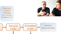

Related Videos:


Select a Web Site
Choose a web site to get translated content where available and see local events and offers. Based on your location, we recommend that you select: United States.
You can also select a web site from the following list
Americas
- América Latina (Español)
- Canada (English)
- United States (English)
Europe
- Belgium (English)
- Denmark (English)
- Deutschland (Deutsch)
- España (Español)
- Finland (English)
- France (Français)
- Ireland (English)
- Italia (Italiano)
- Luxembourg (English)
- Netherlands (English)
- Norway (English)
- Österreich (Deutsch)
- Portugal (English)
- Sweden (English)
- Switzerland
- United Kingdom (English)