When to Use the Hodrick-Prescott Filter
Explore the business cycle filters available in Econometrics Toolbox™ by comparing and contrasting approaches to business cycle analysis over decades of economic research. Filters discussed include the Hodrick-Prescott filter (hpfilter), the Baxter-King filter (bkfilter), the Christiano-Fitzgerald filter (cffilter), and the Hamilton filter (hfilter). Each is described in detail using real-world historical data available with Econometrics Toolbox. The discrete Fourier transform evaluates relative filter performance using a periodogram.
Published: 6 Mar 2023
My name is Bill Mueller. I'm a developer for Econometrics Toolbox at MathWorks, here to talk about when to use the Hodrick-Prescott filter.
So the Hodrick-Prescott filter is what we call a business cycle filter. It's one of four business cycle filters that are available in Econometrics Toolbox as of the 2023a release of MATLAB.
Each of these four filters performs a similar function, and each of these four filters has a similar interface, as indicated at the bottom of the slide here.
The filters take as input an array of data y, representing some macroeconomic time series, and then returns as output a trend component and a cyclical component, such that these are an additive decomposition of y. That is, the trend component plus the cyclical component will always equal y, the original data for all four of the filters.
Now given this similar functionality, the main question that we're going to try in answer in this example is, how do you distinguish these four filters? How do you decide which one to use for a particular application?
And we'll talk about this in various ways. We'll give a little bit of the historical development about where HP filter came from in the first place, how it preceded these other filters, and then how the subsequent filters were, in a sense, a response to the discussions that were generated by the HP filter about how to better capture business cycles in the cyclical output.
We'll see that there are different ways of looking at these filters. The HP filter originally focused on the trend component, using ideas from the part of economics called growth theory, trying to figure out what a reasonable way to compute a trend would be. And the subsequent filters we'll see focus more on the business cycle output here, which is the difference between the trend and the data, by defining and then refining the definition of business cycle in various different ways.
So what we'll see in the end is that the filter you choose has a lot to do with what you're trying to capture in the business cycle. And you can use any one of these filters individually to do a very specific job and capture a very specific notion of business cycle. Or you can use them all together and do a comparative analysis. But we'll talk a little bit about what are meaningful comparisons for these four different filters that have different objectives.
To do this, we're going to look at a live script in MATLAB. A live script is just an MLX file. We're going to look at this when to use the Hodrick-Prescott filter.mlx file. MLX files are files that you can open up in the MATLAB Editor. You can include text and code and then include the outputs from the code, numerical outputs, graphical outputs, right in the display and create a kind of narrative or a presentation of a series of ideas.
So live scripts are handy for comparing and contrasting these different filters. Here's the live script we're going to be looking at. And this live script, together with the slides that we were just looking at, and this recording, are all available on the MathWorks website.
So I'm just going to kind of go through this example at a high level and tell you what's here. And then you can come back to it if you'd like and look at some more of the details.
At the top here, we just introduced the four different filters that we're going to be looking at. There are references to the original research papers which are in a bibliography at the end of this example, and then the names of the functions in Econometric Toolbox that implement these different filters.
Also, just to note that the data that we'll use for this example are data sets that ship with the Econometrics Toolbox. They're historical data that we put in the Toolbox for people to calibrate their models and do prototyping of whatever work they're doing. They're perfectly representative of the kinds of economic data that you would use these filters for. So they'll allow us to demonstrate how these filters work.
If you'd like more up to date data, we recommend going to the FRED database-- the Federal Reserve Economic Data database that's maintained by the Federal Reserve Bank in Saint Louis, at this website.
So to begin, we need to at least ask the question, what is a business cycle? And we'll see that answering that question is much of what this example tries to do. And we'll see that there are different ways that you can answer this question.
Big picture, though, we want to think about all the different forces that are acting on the macro economy. Some of them are very short term. So for example, seasonal effects or interventions of one type or another produce irregular high frequency variations in economic data.
And there are other forces on the economy that are much more long term that produce long term growth and trends in the data. In the discussion of business cycles, which goes way back in the history of economics, is to try and separate in time series that represent macroeconomic data, try and separate out the trend component from these irregular components around the trend that represent cyclical behavior.
Now we want to be careful, then. Cyclical and business cycle suggests a kind of periodic or deterministic behavior. And that's not the case for any of the empirical cycles that we'll be looking at. In real data, the cycles that we'll be discussing are generally non-deterministic and aperiodic and very irregular, with a mixture of many different frequencies.
And that's the challenge of developing these filters, to decide what part of all that you want to separate out and call the business cycle, and what part you want to have remain for the trend.
So just to start us off, we're going to load some data and take a look at it. Here, we're going to look at the US unemployment rate over a period of a number of years and plot it here. Again, I won't go into all the details of the code here. We'll just kind of look at the results. If you want to look at the details of the code, I encourage you to do that.
But here, we have a plot of the US unemployment rate between 1955 and about 2000. Overlaid using this recession plot coming in here are these gray bands that represent historical recession periods in the economy, as determined by the National Bureau of Economic Research, which has for a long time been the final arbiter of what constitutes the beginning and the end of a recession period in the US economy.
So you can overlay those here. And you can see that the unemployment rate generally has a sharp upturn during these recession periods, and then a more gradual downturn during the expansion periods between the recessions, like this.
But there is a, in quotes, cyclical behavior here that you can see, and perhaps a kind of underlying trend as well. And what economists seek to do with data sets like this is try to separate out a notion of trend in this data and a notion of cycle that's going to be meaningful.
As I mentioned, and as is discussed here, there's a long history of how to do this and what's the right way to do this, and how we separate out trend in cyclical components in economic data. The most detailed study of US business cycles in the modern era was originated by a pair of economists named Burns and Mitchell after the Second World War.
They worked for NBER, the National Bureau of Economic Research. And their method was to have a researcher identify the peaks and troughs that they saw in the data, and then compare the data to a series of reference charts that they provided to allow you to determine the periods of the cycles that you saw in the data.
This was used for a long time by NBER to determine where the business cycle was in aggregate macroeconomic data and to determine the turning points in the data and the beginning and the end of recession periods. But the whole methodology was very hands-on and expert oriented. You had to be able to use their reference charts and compare them to the data in order to figure out what the business cycle was.
And they had-- Burns and Mitchell-- had a very definite notion of what a business cycle should be. They said it should be a cyclical component that is no less than six quarter, or 18 months. So nothing shorter term or higher frequency than that, like seasonal effects, but no more than 32 quarters, or eight years. Anything longer than that would be something that would be probably better represented in the trend component than a cyclical component.
So they had this. By looking at a lot of macroeconomic data over a long time, they came up with this very particular idea of what the limits on a business cycle should be kind of this middle frequency data in a time series, between the high frequency seasonal and irregular components and the low frequency components that represented trending behavior.
The problem with this approach, as detailed and insightful as it was about macroeconomic time series, it wasn't very well adapted to modern computer analytics. And this is where the Hodrick-Prescott filter comes in.
So in the '70s, Hodrick and Hodrick and Prescott were two researchers who also worked at NBER, but were interested in using these new computers to come up with a version of the Burns and Mitchell methodology that could be used on computers, easily applied to a lot of different macroeconomic time series, and easy to see how it was creating the outputs.
So there's a discussion here about how they set up the problem as a kind of optimization problem, with their focus being on the trend. What components in the data should constitute the trend? So they're coming from a growth theory perspective, and there are some quotes here from the Hodrick-Prescott paper, the original paper.
They put out a working paper in 1980 describing their filter. And it was much discussed in the econometrics community for decades, until they finally published it in 1997.
During that time, we'll see, the discussion that it generated resulted in these other filters that were going to be going to be comparing it to. But the main point is that the Hodrick-Prescott filter tries to minimize a numerical second derivative, which is represented here, so that the trend component does not vary too quickly.
So it's trying to find a trend component that minimizes this numerical second derivative, and essentially smooth the data, using a known statistical smoothing technique to extract the trend component. And then everything left over, the difference between the data and the trend, would be called the cyclical component.
So in this sense, the Hodrick-Prescott filter was what is now called a high pass filter. It extracts a low frequency trend through smoothing, and then throws everything else into the cyclical component, anything of higher frequency.
The degree of smoothing is determined by a parameter in this optimization, lambda here, which is called the smoothing parameter. And one of the controversies about the Hodrick-Prescott filter that generated a lot of discussion was, how much smoothing do you do to get an accurate representation of the trend? What is the correct way to set this smoothing parameter in order to extract the trend component and get the cyclical component out?
And a lot of discussion has gone into that over the years about appropriate smoothing parameters. The help and documentation for the Hodrick-Prescott filter in Econometrics Toolbox offers some suggestions for smoothing parameters that are recommended by different researchers for data with different periods, whether it's quarterly, annual, monthly, et cetera. But you can play around with it too in the documentation by tuning the tuning parameter the smoothing parameter and seeing the different kinds of trends that you get.
So with that background, let's just take a look at the HP filter function in Econometrics Toolbox. We're going to look at this unemployment data that we just looked at and apply the HP filter to that data, setting the smoothing parameter to what Hodrick and Prescott recommend for quarterly data, which is what the unemployment rate data is.
And we're going to compare that to applying the HP filter to the same data, but with a much more aggressive smoothing parameter. This smoothing parameter was suggested by more recent researchers, Robin and Uhlig, who re-examined in 2022 the Hodrick-Prescott filter and made arguments in their paper about why more aggressive smoothing parameters were maybe appropriate for finding the overall trend in the data and getting a more accurate cyclical component out as a difference.
So we're going to play two different smoothing parameters here to the unemployment rate data. And the result looks something like this. The HP trend, with the original smoothing parameter suggested by Hodrick and Prescott, is this solid red line overlaid on the data. And the Ravn-Uhlig trend, with the more aggressive smoothing parameter, is this dotted magenta line here.
And you can see that it does smooth the data more than the smaller smoothing parameter that Hodrick and Prescott uses. If we look at the difference between the trend in the data, we arrive at the cyclical components, and we get this graph, color coded in the same way.
And you can see, because the Hodrick-Prescott smoothing parameter is less aggressive, the deviations from the data, the cyclical component, are smaller, in general, than the deviations when you use a larger smoothing parameter like in the RU data here.
So that's a little background on the Hodrick-Prescott filter, where it came from, and how it's used. It involves setting this smoothing parameter. And again, that's debatable about what the value of that smoothing parameter should be.
So let me move on to some of the other filters that came about in the decades between 1980, when Hodrick-Prescott first introduced this filter to the econometric world in 1980 and the couple of decades that went by until they finally published a paper. There was a lot of discussion about whether this was the correct way to capture the trend in the data, or whether this was the correct way to capture the business cycle in the data.
Note that the hot the Hodrick-Prescott filter does not try-- it never did try to define what a business cycle was. It was just focused more on smoothing and defining the trend in the data. And passing all the higher frequency components into what was left over, was called the cyclical component.
It wasn't trying to match some definition of business cycle. And that's what generated much of the discussion after the Hodrick-Prescott filter came out. There were a lot of papers written about the Rick Prescott filter and alternatives to it.
One of the alternatives to the Hodrick-Prescott filter that came to be most highly regarded was the Baxter and King filter that came out in a paper in 1999. The difference between the Baxter-King filter and the Hodrick-Prescott filter is that the Baxter-King filter has a very specific notion of what a business cycle should be.
And they go back to Burns and Mitchell and say what the filter should do to get a business cycle out-- not just all the high frequency components, but a business cycle. What it should do is act as a bandpass filter and filter out all of the low frequency components that are usually assigned to the trend, but also filter out high frequency components that represent seasonality and these irregularities that come from aggregating data and so forth.
So they developed, in the way that somebody in signal processing might, a bandpass filter, or an approximate bandpass filter, where you can specify lower and upper cutoff periods. And the filter attempts to, with the limited amount of data that you're always going to have, attempts to filter the data to only include the middle frequencies between those two cutoffs in the business cycle.
And their defaults are to use the Burns and Mitchell cutoffs of six months and eight-- the Burns and Mitchell that we saw earlier here. Between six quarters and 32 quarters, or eight years, were the two default cut-offs that they wanted to work with.
But of course, those are parameters that are used in the filter. And you can set those cutoff periods to whatever you choose to make your own definition of business cycle.
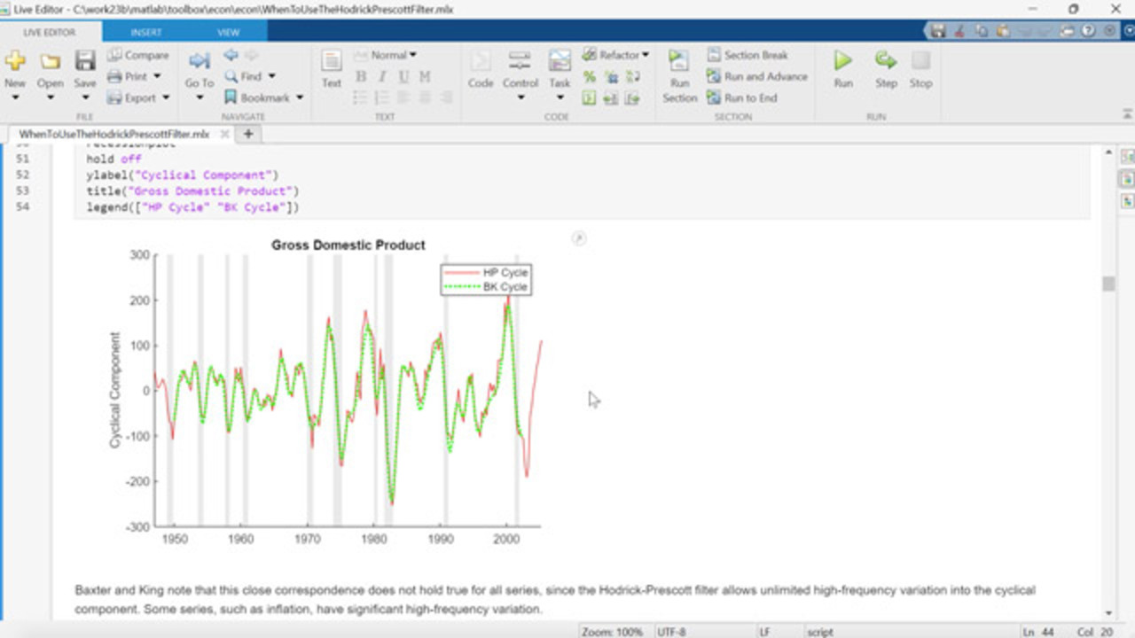
So let's just take a look at how the BK filter looks in practice. We're going to load some new data here on the gross domestic product, the output in the US economy. And this has quarterly data. We're going to plot this GDP data. We see, it has a definite trend to it, and then some sort of cyclical component around the trend. And the Baxter-King filter is going to try and separate these two.
We'll compare it to the HP filter directly by, on the same data, applying the HP filter and the BK filter to the same data and plotting it. And what we get is something that looks like this. We can see that even though the approaches are very different between the HP filter trying to use smoothing methods to determine a trend, and the BK filter, which is acting as an approximate bandpass filter, the results are much the same.
And Baxter and King noted this, that even though their very specific notion of business cycle was different than that of Hodrick and Prescott, for many macroeconomic time series, they produce remarkably similar results.
But as Baxter and King noted, the difference is that the Hodrick-Prescott filter passes all high frequency components into the cyclical component, whereas the Baxter-King filter trims off a certain amount of the high frequency that's outside of the band that it defines.
So if there is a lot of high frequency, if there's a high frequency component in the data, it's probably going to show up more in the HP cycle than it is in the BK cycle. And there are economic time series that involve very high frequency data. The example we look at here is the inflation rate.
So we take the consumer price index and compute a version of the inflation rate. The inflation rate typically has very high frequency variation.
And then we apply, in the same way as we did up above, both the HP filter in the BK filter to this inflation rate data. And in this case, you can see that the absolute deviation in the Baxter-King cycle is much smaller than it is in the HP cycle. The HP cycle is picking up all of this high frequency, high end stuff that gets trimmed by the Baxter-King filter. And you see a difference here.
So here, we get two different business cycles. Again, Hodrick and Prescott might argue that they were just capturing the cyclical component and not specifically a business cycle. But their cycle and specifically business cycle of the BK filter can differ, as we see here, especially when there's a high frequency component in the data.
So right there, you have a distinction between the Hodrick-Prescott filter and the Baxter-King filter. Which one would you use? Well, if you want to come up with a nice trend through statistical smoothing methods, the HP filter is designed to do that, just putting everything else into the cyclical component.
The Baxter-King filter, on the other hand, tries to work with the Burns and Mitchell definition of a business cycle and trims out the low frequency and the high frequency components to give you the middle frequencies in the business cycle. And you can determine what that middle is by setting the cutoff parameters in the Baxter-King filter.
Not long after Baxter and King put out their paper on a bandpass filter for commuting business cycles, Christiano and Fitzgerald followed up with another version of a bandpass filter. Same idea, that they were going to cut out low frequencies and cut out high frequencies and identify the business cycle as something in the middle, using the same defaults as Burns and Mitchell's, same idea as what Baxter and King suggested.
But the mathematics was a little different. They-- Christiano and Fitzgerald, as it says here, they optimized a different objective function in order to come up with their trend and cycle. But it didn't operate in a different way than the Baxter-King filter.
You specify the two cutoff frequencies, and you apply the filter. And you get some middle frequency data. The Christiano-Fitzgerald filter was specifically designed, it says here, to produce asymptotically optimal finite sample approximations to an ideal bandpass filter, something the Baxter-King filter didn't specifically address.
So the idea being that the more data you have, asymptotically, the closer this filter would come to an ideal bandpass filter, with step function cutoffs at the two cutoff frequencies.
In order to do this, in order to make this optimally designed filter, they had to make an assumption that, as it says here quote from their paper, the filter was optimal under the most likely false assumption that the data are generated by a purely random walk. That is, that the data have a unit root in them.
And as discussed a little bit in the example here, the idea of whether there are unit routes in economic data is another long, ongoing debate. Whether the data have unit roots or not has serious implications for doing things like forecasting, which is one of the things that people extracting business cycles are most interested in.
So there is an ongoing discussion about the possibility of this assumption being true or being false-- in particular, economic data. But what Christiano and Fitzgerald also argue later-- and it's quoted here in the example-- is that even if this assumption is false, that for a large number of economic time series, their filter performs very well. So it may not be optimal. But it performs very well in its bandpass-- it's self-described bandpass goal.
So in order to evaluate it, what we do here is, we create a random walk, a random walk just being an autoregressive series with the autoregressive coefficient being 1 here. That's the unit root. We're going to add a drift component, and then some random innovations here to the data.
And if you look at a random walk with a drift, you get data that looks something like this, looks much like the GDP data that we just looked at-- the GDP data, of course, being empirical. This is just simulated data of simulated random walk. But it's data that meets the assumption that Christiano and Fitzgerald made that allowed them to prove that their filter was asymptotically optimal.
So just looking at this data, treating this data as quarterly, say like we did the GDP data, we can apply the Baxter-King filter and the Christiano-Fitzgerald filter to it. We have to set this drift parameter equal to true in the CF filter. It's an additional parameter here, that you have to specify whether you're working with data that has a drift or not. That's not required in the Baxter-King filter.
And we can see, if we look at the results, that the Baxter-King and Christiano Fitzgerald filter are similar on this scale, in terms of the cycle that they extract. So they're two different versions of a bandpass filter. You can see that the BK filter trims data at both the beginning and the end of the data. That's because it uses a fixed lag length to create a moving average that smooths the data when it's computing the trend, whereas one of the innovations in the Christiano-Fitzgerald filter is that it uses a moving average that changes size as you move through the data and allows you to compute the moving average for the entire data set to extract the trend.
And so it doesn't need to do trimming. So that's certainly an advantage of using the Christiano-Fitzgerald filter.
If we look at real empirical data, again, Christiano and Fitzgerald claiming that their method is nearly optimal for many types of time series representations that fit US data on interest rates, unemployment, inflation, and output. They claim that even if you aren't looking at data that has a unit root or is a purely random walk, that it still works well.
And to check that out, we just go back to the empirical GDP data here and compare the BK filter and the CF filter on this data, and see that again, we get similar results, maybe with the CF filter giving slightly higher amplitude excursions in the cycle. And of course, those high amplitude changes in the cycle are typically what are used to date periods of recession and expansion, beginning and end of them.
So potentially, the inference that you would draw from where to date the business cycle would be different from these two filters if the amplitudes of the cycles are significantly different. And they can be, depending on what particular data you look at.
So just in summary, the Baxter-King filter and the Christiano-Fitzgerald filter are coming from the same place. They're both bandpass filters. They have slightly different mathematical foundations or goals, and of course, different algorithms then that compute the cycle.
But they both functionally behave the same way, in that you give cutoff periods at the low end and the high end and collect the middle frequency data in the cyclical component for the output here. And depending on the data you look at, they can be more or less different. But they're often used together, honestly, in most econometric research to compare them with their two different optimizations and their are two different approaches to bandpass filtering, to get different takes on where these business cycles begin and end.
Now there's another take on the Hodrick-Prescott filter. In 1999, the researchers Stock and Watson looked at the Hodrick-Prescott filter and said it was problematic, in terms of doing forecasting of the business cycle.
And part of the reason for that is that there was that arbitrary smoothing parameter that we talked about earlier and how to set it. But also, if we go all the way back and look at the objective function that gets optimized in the Hodrick-Prescott filter, notice that this derivative that it's calculating involves not just values at time t at any point, but subsequent values and previous values.
So it's what's called a two sided filter. It's looking at data both before and after time t at any time t in order to compute this derivative and then do the optimization. So it's called a two sided filter.
And it's also-- and this is what Stock and Watson were focusing on-- it's also non-causal, in the sense that at time t, if you're working in real time, you generally won't have data on time t plus 1. And so you won't be able to apply this. And for that reason, the Hodrick-Prescott filter is typically used on historical data, where at any time t you have both the data in front of you and the data behind you.
But for real time forecasting, Stock and Watson say that can be problematic. That can create end effects where the data, the cyclical output has artificial predictive power. Because it's using data in the future.
And so they propose what's called a one-sided Hodrick-Prescott filter that does much the same thing as the Hodrick-Prescott filter, but computes that derivative using only current and past data. In other words, the filter is causal. It's one sided and causal. It can be used in real time. It doesn't update the outputs when new data is acquired.
And they make an argument in their paper that that's a much better way of computing the trend and cyclical component if your objective is to do forecasting. And often, that's the case.
So if you want to look at the Stock and Watson implementation of the one-sided Hodrick-Prescott filter, you can still use the HP filter function. But, and you can still set the smoothing parameter. But there's a filter type parameter here that can be set to either one-sided or two sided.
If you set it to one-sided, you get the Stock and Watson filter. If you set it to two-sided, you get the original Hodrick-Prescott filter. And you can run them both on, say the GDP data, as we do here. And you can see that they do indeed provide different cyclical outputs for the GDP data.
And that could be significant if your goal is to fit a model to this cyclical data and then forecast from that model into the future. Of course, fitting to these different cycles is going to result in different model parameters and different forecasts. And you do get different results. We'll compare those forecast results here in a moment, in the example.
Finally, the fourth filter that we want to compare here is what's come to be called the Hamilton filter, introduced by James Hamilton, a well known economist. He wrote a paper in 2018 that had a very provocative title, called Why You Should Never Use the Hodrick-Prescott filter.
And Hamilton goes on to express some of the same concerns that Stock and Watson did about forecasting abilities, that there are different smoothing parameters you can set in the Hodrick-Prescott filter, different ideas about what are the right ones to extract the trend, the fact that the two-sided filter created these end effects that affected forecasting, and that maybe gave unrepresentative results when you did the forecasts.
And so again, he has this very strong title, that you should never use the Hodrick-Prescott filter. But as we've already discussed, a lot of the concerns that Hamilton has raised have been addressed by previous researchers, in terms of how to deal with better forecasting capability and how to set the smoothing parameter based on different assumptions.
But we should note too that Hamilton is focusing on a goal, a definition of business cycle that's different from what Hodrick and Prescott had set out in the first place, Hodrick and Prescott looking for a way to use statistical smoothing to come up with a reasonable trend, and Hamilton kind of changing the playing field and saying, what we really want to do is be able to create a good forecast, which is perfectly reasonable, but wasn't expressly what Hodrick and Prescott had set out to do.
So Hamilton claims that there is a better alternative than using the Hodrick-Prescott filter. In essence, he says that you can perform a simple linear regression, causal regression using, at any time t, the most recent observations in a time series as predictors to create a linear regression model, forecast that forward in order to get a forecast result, and then use the difference between the forecast and the actual data, the forecast error, to represent the business cycle.
So Hamilton has a very specific definition of business cycle too. It's the forecast error from the regression model that he suggests. It's nothing like the Baxter-King or the Christiano-Fitzgerald definition of business cycle, which is a bandpass version of the business cycle based on the Burns and Mitchell research.
But he says that this is a much better way to use the filter to come up with trends and cycles for forecasting applications. Fair enough. It's good for that. But it's a different definition of business cycle.
So we can implement Hamilton's idea. We do in this H filter function in Econometrics Toolbox. It requires you to specify a couple of parameters-- a lead length, how far out do you want a forecast from this regression model in order to calculate the forecast error and get the cyclical component, lag length, how far back do you want to go in the data in order to get predictors in this regression model. And there are defaults that are set for this, of course.
And we can apply the Hamilton filter and the one-sided Hodrick-Prescott filter and compare them. It makes sense to compare these two, because both the Hamilton filter and the one sided Hodrick-Prescott or the Stock and Watson filter have as their self stated objective to come up with good forecasting performance.
So if we compare those two, we see that we get similar, but on this scale somewhat different cyclical components, with the Hamilton cycle showing much sharper departures during the periods of recession.
Now, that could be considered a very good thing. Because these departures are what are used to date to date the start and end of a particular recession period. So a sharp departure is going to be more distinctive and maybe help to identify those departures better than a smaller departure. So in this case, with the GDP data, you could argue that the Hamilton filter does do a better job of identifying those turning points in the business cycle.
And of course, when you're fitting, then, a forecasting model to this data, you'll get different results. And we'll compare those here in a minute.
All right. So we talked about all four of the different filters, including the two versions of the Hodrick-Prescott filter that are in the Econometrics Toolbox. We talked a little bit about the history and how they evolved, one trying to address issues with previous filters, how they had different definitions of what the trend component or the business cycle component should be. And hopefully, some of that discussion is helpful in choosing which filter you would want to use for a particular application.
If we want to evaluate how good are each of these filters at actually determining the business cycle, that's a harder problem. And the main point in this final section is that the reason that's a hard problem is because we will never know what the true business cycle is. We don't have empirical data ever on just the business cycle that we can compare with the outputs from these different filters.
The business cycle is more of an idea, a component in some data generating process out there that's creating all of this macroeconomic data. We don't have that data generating process. We can estimate it. We can model it with different models. But we never know exactly What it is.
So an absolute evaluation of any of these filters, about how well do they capture the business cycle, is really impossible. Because we don't know what the business cycle is, and each of these filters has a different goal, a different idea of what the business cycle should be.
However, we can look at the relative performance of these different filters. If the two, if two filters have similar goals, we can take them at their word and compare them with respect to those similar goals.
For example, the Baxter-King and Christiano-Fitzgerald filters are both bandpass filters, supposed to capture a business cycle between two frequencies or two periods in the data. And we do here a comparison of those two filters on the GDP data using a power spectrum.
So what we're going to do is, we're going to calculate the Fourier transform of the business cycles that are output from each of these filters and use those to calculate the power spectrum of how much power is in the data at each different frequency, looking just at the cyclical component that comes out and creates something called a periodiogram that displays the power in the business cycle at different frequencies.
This is all signal processing kind of terminology. But it's used in econometrics quite a lot, when you're looking at things in the frequency domain. And this is just sort of the standard approach for taking Fourier transforms in MATLAB and creating a power spectrum. It's not hard to do.
And we can plot the power spectrums, get the periodiogram, and see that if these red lines represent the cut-off periods, or the cut off frequencies in this case, that are specified for both filters-- it was identical in both calculations-- that indeed, most of the power in this spectrum is within the band, in the bandpass filter, as it should be.
They're both trying to say that the frequencies that represent the business cycles are the frequencies between these two delimiters. Both of these bandpass filters are trying to filter out these low frequency components and these high frequency components.
And we can see that, again, it's kind of apples and oranges, that for this particular data, this GDP data, the Christiano-Fitzgerald filter does a much better job of filtering out the low frequencies, the trend data. But in this case, at least, the Baxter-King filter does a better job of filtering out some of the high frequencies, the things that would be dumped into the cyclical component in a Hodrick-Prescott cycle.
So a periodiogram like this is a good way to compare two filters that have the same objective, which is to only output in the cycle the frequencies that are between some low end and some high end.
Likewise, if we want to compare, say the one-sided Hodrick-Prescott filter and the Hamilton filter, which have similar goals-- they're both supposed to be designed to improve forecasting performance-- we can-- and I won't go through all of this code. But it's-- quickly, what it is is it takes the GDP data, breaks it up into-- takes the first 2/3 as a estimation part of the data, an estimation sample, and retains the last 1/3 of the data as a forecast sample, fits a model to the estimation sample-- this is sample of the cyclical component that comes out of both of the filters, the one-sided Hodrick-Prescott and the Hamilton filter.
The model we're going to fit here is a Markov switching model, which is often used for simple two state recession expansion models. And we fit a Markov switching model here to both cycles. That's what this is, and then use the forecast methods to forecast from those cycles into the final 1/3 of the data, and compare, over that horizon, compare the forecasts to the actual data.
So we're going to take the two cycles, fit a Simulink model to both cycles, as defined by the two different filters, and then compare their forecast performance there. They're both claiming to be good at that.
And so the black data here is the Hamilton cycle, both in the estimation period and the forecast period. The red dotted data is the one-sided Hodrick-Prescott cycle in the estimation period and the forecast period. And then the solid lines represent the point optimal forecasts.
There are different ways you can forecast ahead. These are the-- we applied the optimal point forecast, looking into the forecast horizon here.
And you can see that they do give different forecasts, looking ahead here. But they're more or less comparable on this scale for this data over this horizon. So does one do better than the other? That's really hard to say without knowing what you want to do with these forecasts there.
They're very similar in this case. But it's hard to evaluate whether one filter, the cycles that we're using to do this forecasting is better than the other. Because these forecasts depend first of all on the model we chose to fit this particular two state Markov switching model, and also on the method that we used for forecasting. There are different ways for forecasting.
So depending on the model you use and depending on the forecast method, each of these cycles will produce different forecasts. So it's not as simple as one cycle is better than the other. They're different. And it's really going to be up to the researcher looking closely at the data to make a determination about which of these cycles to use.
Finally here, we're going to give Hodrick the final word. In 2020, after Hamilton published his paper saying to never use the Hodrick-Prescott filter, Hodrick published a rebuttal, where he very carefully looked at a number of different data generating processes, a number of different models of how data and the economy gets generated, all of them that are widely used for modeling economic data.
And he looked at things like ARIMA models and random walks, as we already have, and then also at more complex models, where these things that are called unobserved component models, where you can specifically say, here's the trend component in the data generating process. Here's the cyclical component, and put them together.
So this code is going to using parameters that Hodrick has estimated from GDP data. This is going to be an unobserved components model with a cyclical component here and a trend component here. And the data is going to be the sum of the simulated cycle and the simulated trend.
Now you can argue about this, whether this is representative of true economic data or not. But it's data with a built-in cyclical component and a built-in trend component. And so we can compare, if we apply the filters to the data itself. We can compare the cycles that are output and the trends that are output to the cycles and trends in the data generating process, something we can't do in the true economy, but we can do in a simulation like this. So it gives us something of an absolute comparison between the different filters on the simulated economic data.
And what this produces, using, again, parameters that Hodrick has estimated, using GDP data, it gives us simulated GDP data that looks something like this. And we can run this multiple times to get different simulations and perform statistical analyses on all of this.
And we can apply the HP filter, the original HP filter, the Baxter-King filter, just to put a band pass filter in there for comparison, and the Hamilton filter, all to the simulated data, extract the cycles, and then compare the cycles to that simulated cycle that's in the data generating process.
So the simulated cycle is this dark blue cycle, and these other lines are the cycles that are output from the different filters, applied to the data as a whole-- the trend plus the cycle.
And you can see, all of them seem to approximate the cycle in the data generating process. The Hodrick-Prescott and Baxter-King filter follow each other much more closely. And once again, we see that the Hamilton filter has much more distinctive swings at the upturns and the downturn, which could be useful for identifying turning points in the business cycle.
Another way to compare these is just look at the pairwise correlations of these different cycles, which we do here using the core plot command in Econometrics Toolbox. And you can see here with the core plot here, we've got the different series labeled on the axes-- our the different filters, rather.
And we can see, if we're looking at, say the correlation between the Baxter-King and Hodrick-Prescott cycles and their data, we have a very high correlation, 0.97. But if we look at the correlation between, say the HP filter and the Hamilton filter, which would be here, we get a much lower correlation.
And the correlation between the actual data generating process and the Hamilton filter is lower than it is for the Baxter-King filter or the HP filter. We get a correlation coefficient of about 0.85 for both the HP and the BK filters, but a correlation coefficient of only 0.62 for the Hamilton filter.
So Hodrick's point in his paper here is that-- well, I'll read his summary here. He says, consequently, the most desirable approach to decomposing a time series into growth and cyclical components, and hence the advice that one would give to someone that wants to detrend a series to focus on cyclical fluctuations, clearly depends on the underlying model that one has in mind. For GDP, if one thinks that growth is caused by slowly moving changes in demographics, like population growth and changes in rates of labor force participation, as well as slowly moving changes in the productivity of capital in labor, then the filtering methods of Hodrick and Prescott and Baxter-King seem like the superior way to model the cyclical component.
And by superior, he's basing it on evidence such as this about how well the different filters capture the true cycle in simulated economic data like this.
So to sum up, and to rebut Hamilton, what Hodrick finally concludes is, that to my way of thinking, the title of the Hamilton paper, which was Never Used the Hodrick-Prescott Filter-- is clearly too strong. And I think that's accurate.
We talked in this example about when to use the Hodrick-Prescott filter, rather than never use the Hodrick-Prescott filter. And we've seen that it's valuable in a lot of different circumstances for a lot of different time series, just as the Hamilton filter is valuable for certain applications, and the Baxter-King and Christiano-Fitzgerald filters, depending on your objectives.
So all of this is summarized at the end here, about what the different filters focus on and why you would pick one instead of the other, or how you can use them together to do a more comparative analysis. And I hope that this has helped you to start to distinguish among these four filters and think about how you might want to use them to do your own analysis.
At the end here, I'll just note that there's a reference section with references to all of the different authors and papers who have participated in the discussion of business cycles and business cycle filtering over the last 40 years or so, since Hodrick and Prescott first put out their filter.
I'll also mention that we have quite a lot of documentation that's available at the MathWorks website or with an installation of MATLAB, in the Econometrics Toolbox. Lots of documentation.
Here's a link to the documentation for the Econometrics Toolbox, examples of-- more examples of how to use each of these filters, how to tune the different parameters. Get into this in much more detail.
So thank you for listening, and I hope this was helpful to you for doing your own business cycle analysis.
Download Code and Files
Related Products
Learn More
Featured Product
Econometrics Toolbox
Up Next:


Related Videos:


Select a Web Site
Choose a web site to get translated content where available and see local events and offers. Based on your location, we recommend that you select: United States.
You can also select a web site from the following list
Americas
- América Latina (Español)
- Canada (English)
- United States (English)
Europe
- Belgium (English)
- Denmark (English)
- Deutschland (Deutsch)
- España (Español)
- Finland (English)
- France (Français)
- Ireland (English)
- Italia (Italiano)
- Luxembourg (English)
- Netherlands (English)
- Norway (English)
- Österreich (Deutsch)
- Portugal (English)
- Sweden (English)
- Switzerland
- United Kingdom (English)