Evaluate 3GPP Indoor Reference Scenario

R2026b

Since R2024a

This example uses:

This example shows how to model, simulate, and evaluate the system-level performance of a 3GPP enhanced mobile broadband (eMBB) indoor hotspot (InH) scenario, described in 3GPP TR 38.913.

Using this example, you can:

Create an eMBB InH scenario representing a single floor of a building.
Create and configure base stations (gNBs) and user equipment (UEs).
Connect UEs to the gNBs, and add full buffer uplink (UL) and downlink (DL) application traffic between them.
Configure and add a scheduler and channel model.
Run the simulation, and visualize the key performance indicators (KPIs) such as cell throughput, spectral efficiency, and block error rate (BLER).

Additionally, you can use this example to perform these tasks.

eMBB InH Reference Scenario

This example models and simulates an eMBB InH scenario consisting of a single floor within a building.

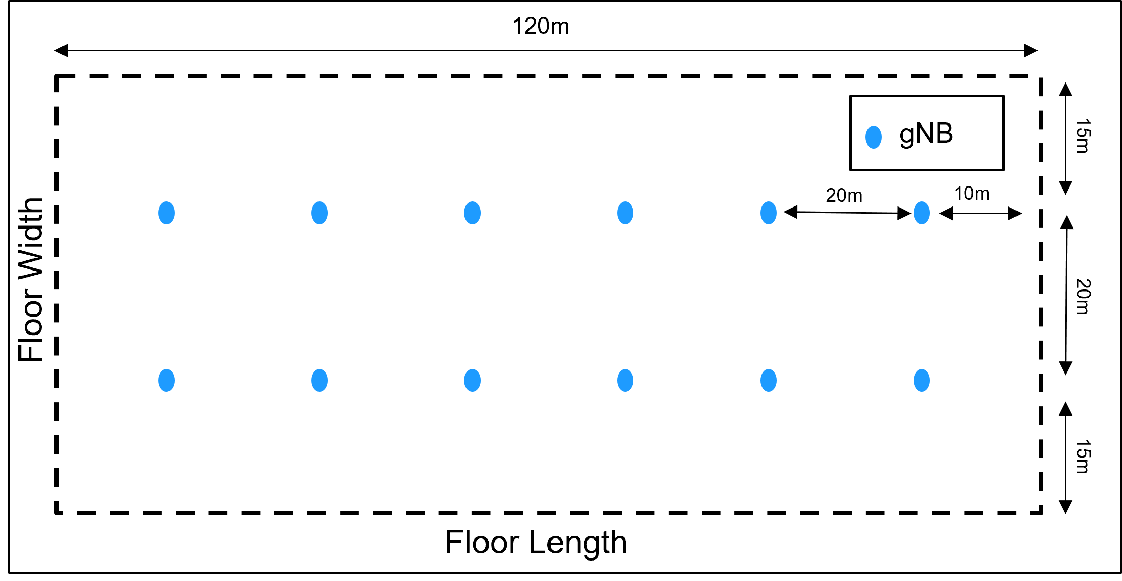
These are the specifications of the scenario:

Floor dimensions — The scenario consists of a rectangular floor 120 meters in length and 50 meters in width. The ceiling height is uniformly set at 3 meters throughout the floor.
gNB distribution — Twelve gNBs, also known as sites, are strategically placed throughout the floor area. The gNBs are organized in a grid layout, each spaced 20 meters apart, to ensure complete coverage within the indoor scenario.
UE distribution — The scenario allocates 10 UEs to each gNB within the indoor scenario. The distribution of UEs is intended to be random, confined to the area delineated by the location of each gNB.

The indoor scenario has been modeled to cover a variety of typical indoor environments, including office spaces and shopping centers. The scenario accurately simulates common office layouts, incorporating features such as cubicles, walled private offices, expansive open areas, and corridors. Depending on your simulation requirements, you can configure the channel model as "Open" or "Mixed".

"Open" — The Open Office environment consists of a large open space with minimal obstructions, like an open-plan office area. The signal propagation is relatively uniform, and the user distribution is typically even. This scenario is used to model high-capacity areas, where you expect many users to access the network simultaneously.

"Mixed" — The Mixed Office environment is more complex, consisting of a combination of open areas and closed offices with walls and partitions. The user distribution is more varied, and the signal experiences more multipath fading and shadowing effects. Use this scenario to model typical office environments, with a mix of open spaces and enclosed rooms.

Simulation Assumptions

In this example, these assumptions apply:

The gNB-UE association is based on the proximity of the UE to the gNB.
A UE connects to the gNB that is nearest to it.
The UEs are randomly placed within a circular area around each gNB.

Configure and Simulate Scenario

Reset the seed value for the random number generator. The seed value controls the pattern of random number generation. To improve the accuracy of your simulation results after running the simulation, you can change the seed value, run the simulation again, and average the results over multiple simulations.

rng("default");

Specify the simulation time in terms of number of 10 ms frames.

numFrameSimulation = 2;

Initialize the wireless network simulator.

networkSimulator = wirelessNetworkSimulator.init;

Configure gNBs and UEs

Specify the frequency and bandwidth at which the carrier served by the gNB operates. The subcarrier spacing in the carrier frequency is 15 kHz.

carrierFreq = 4e9;  % In Hz
channelBW = 10e6;   % In Hz

Specify the number of gNBs in the vertical and horizontal directions.

numVerticalGNB = 2;
numHorizontalGNB = 6;

Specify the number of transmit and receive antennas for the gNBs.

gNBNumTransmitAntennas = 32;
gNBNumReceiveAntennas = 4;

Specify the noise figure and transmit power of the gNB.

gNBNoiseFigure = 5; % In dB
gNBTxPower = 21;    % In dBm

Specify the number of UEs connected to each gNB. According to the 3GPP TR 38.913, a gNB is typically assigned 10 UEs. However, To keep simulation runtime in check, this example uses a default value of 2 UEs per gNB.

numUEsPerGNB = 2;

Specify the number of transmit and receive antennas for the UEs.

ueNumTransmitAntennas = 4;
ueNumReceiveAntennas = 4;

Specify the noise figure and transmit power of the UE.

ueNoiseFigure = 7; % In dB
ueTxPower = 23;    % In dBm

Create gNBs and UEs in each cell of the InH scenario.

scenario = h3GPPReferenceScenarios(Scenario="InH",NumUEs=numUEsPerGNB, ...
     NumGNBsHorizontal=numHorizontalGNB,NumGNBsVertical=numVerticalGNB, ...
     MaxUEsPerGNB=numUEsPerGNB);
gNBCoordinates = scenario.GNBPositions;
ueCoordinates = scenario.UEPositions;

Create gNBs and Configure Scheduler

Create the gNBs from the specified configuration. Each gNB operates one NR cell.

gNBs = nrGNB(Position=gNBCoordinates,NoiseFigure=gNBNoiseFigure, ...
     CarrierFrequency=carrierFreq,ChannelBandwidth=channelBW, ...
     NumReceiveAntennas=gNBNumReceiveAntennas, ...
     NumTransmitAntennas=gNBNumTransmitAntennas, ...
     TransmitPower=gNBTxPower,SRSPeriodicityUE=5);

Compute the total number of gNBs.

numGNBs = size(gNBs,2);

Configure the link adaptation (LA) parameters. The parameters specify a 10 percent target BLER for the UL and DL configurations.

laConfigDL = struct("StepUp",0.27,"StepDown",0.03,"InitialOffset",1,"ResetOffsetOnCSIReport",false);
laConfigUL = struct("StepUp",0.27,"StepDown",0.03,"InitialOffset",1,"ResetOffsetOnCSIReport",false);

Configure the scheduler by specifying the gNBs, maximum number of users per transmission time interval (TTI), and LA configuration.

configureScheduler(gNBs,MaxNumUsersPerTTI=10,...
    LinkAdaptationConfigDL=laConfigDL,LinkAdaptationConfigUL=laConfigUL)

Configure the UL power control parameters.

for gNBIndex = 1:numGNBs
    configureULPowerControl(gNBs(gNBIndex),Alpha=0.6)
end

Create UEs and Configure Application Traffic

Create the UEs from the specified configuration.

UEs = nrUE(Position=ueCoordinates,TransmitPower=ueTxPower, ...
     NumTransmitAntennas=ueNumTransmitAntennas, ...
     NumReceiveAntennas=ueNumReceiveAntennas,NoiseFigure=ueNoiseFigure);

Connect the UEs to the gNB. Configure and add UL and DL full buffer traffic between each gNB and its connected UEs.

startUEIndex = 1;
ueListInGNB = cell(1,numGNBs);
for gNBIndex = 1:numGNBs
    connectUE(gNBs(gNBIndex),UEs(startUEIndex:startUEIndex+numUEsPerGNB-1), ...
        CSIReportPeriodicity=160,FullBufferTraffic="on")
    ueListInGNB{gNBIndex} = UEs(startUEIndex:startUEIndex+numUEsPerGNB-1);
    startUEIndex = startUEIndex + numUEsPerGNB;
end

Add the gNBs and UEs to the wireless network simulator.

addNodes(networkSimulator,gNBs);
addNodes(networkSimulator,UEs);

Configure Channel Model

Specify the channel type as "Open" or "Mixed".

officeType = "Mixed";

Create a system-level channel model for the scenario.

channel = h38901Channel(Scenario="InH",OfficeType=officeType);
chcfg.Site = 1:numGNBs;

Specify the transmit antenna array orientation.

chcfg.TransmitArrayOrientation = [0 90 0]';

Add the channel model to the simulator.

addChannelModel(networkSimulator,@channel.channelFunction);
% Connect the simulator and channel model
connectNodes(channel,networkSimulator,chcfg,InterfererHasSmallScale=true);

Run Simulation and Visualize Metrics

Set the number of updates per second for the metric plots.

numMetricPlotUpdates = 1000; % Updates plots every millisecond

Specify the cell ID for the desired gNB to access its corresponding visualizations and metrics.

cellOfInterest = 1;

To visualize PHY and MAC metrics, create and configure the helperNRMetricsVisualizer object.

metricsVisualizer = cell(numGNBs,1);
for cellIdx = 1:numGNBs
    if cellIdx == cellOfInterest
        metricsVisualizer{cellIdx} = helperNRMetricsVisualizer(gNBs(cellIdx), ...
            ueListInGNB{cellIdx},RefreshRate=numMetricPlotUpdates, ...
            PlotSchedulerMetrics=false,PlotPhyMetrics=false,CellOfInterest=cellIdx, ...
            PlotCDFMetrics=true);
    else
        metricsVisualizer{cellIdx} = helperNRMetricsVisualizer(gNBs(cellIdx), ...
            ueListInGNB{cellIdx},RefreshRate=numMetricPlotUpdates, ...
            PlotSchedulerMetrics=false,PlotPhyMetrics=false, ...
            CellOfInterest=cellIdx,PlotCDFMetrics=false);
    end
end

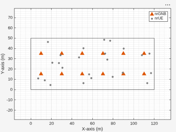
Display the network topology.

networkVisualizer = wirelessNetworkViewer(ShowNodeNames=false);
showBoundary(networkVisualizer, Position=[60 25 0], BoundaryShape="rectangle",Bounds=[120 50], ...
    Name="RectangleBoundary")
addNodes(networkVisualizer,gNBs)
addNodes(networkVisualizer,UEs)

Compute the simulation time from the specified numFrameSimulation frames.

simTime = numFrameSimulation*1e-2;

Run the simulation.

run(networkSimulator,simTime)

Figure Wireless Network Viewer contains an axes object. The axes object with xlabel X-axis (m), ylabel Y-axis (m) contains 73 objects of type line. One or more of the lines displays its values using only markers These objects represent nrGNB, nrUE.

Figure ECDF of Block Error Rate (BLER) contains 2 axes objects. Axes object 1 with title Average Cell DL BLER, xlabel BLER, ylabel ECDF contains 3 objects of type stair, constantline. This object represents Average BLER. Axes object 2 with title Average Cell UL BLER, ylabel ECDF contains 3 objects of type stair, constantline.

Figure ECDF of Cell Throughput contains 2 axes objects. Axes object 1 with title Cell DL Throughput, xlabel Cell Throughput (Mbps), ylabel ECDF contains 3 objects of type stair, constantline. This object represents Cell Throughput. Axes object 2 with title Cell UL Throughput, ylabel ECDF contains 3 objects of type stair, constantline.

Figure ECDF of Application Layer Latency contains 2 axes objects. Axes object 1 with title Average App DL Latency, xlabel Latency (s), ylabel ECDF contains 2 objects of type constantline. Axes object 2 with title Average App UL Latency, ylabel ECDF contains 2 objects of type constantline.

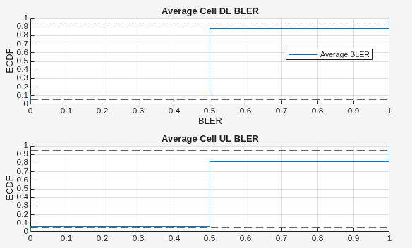
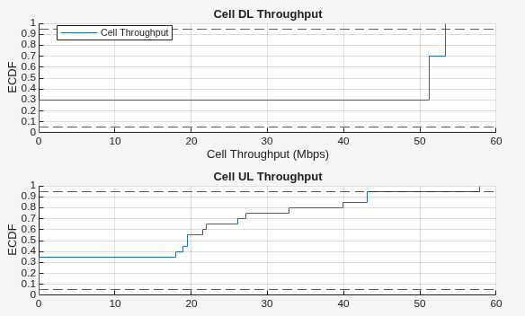
Display the system KPIs for the scenario.

fprintf("\n\nMetrics for site %d:\n\n",cellOfInterest)

Metrics for site 1:

displayPerformanceIndicators(metricsVisualizer{cellOfInterest})

Peak UL throughput: 258.80 Mbps
Achieved cell UL throughput: 19.46 Mbps
Achieved UL throughput for each UE: [8.68        10.78]
Peak UL spectral efficiency: 25.88 bits/s/Hz
Achieved UL spectral efficiency for cell: 1.95 bits/s/Hz 
Block error rate for each UE in the UL direction: [0.5       0.625]

Peak DL throughput: 258.80 Mbps
Achieved cell DL throughput: 36.47 Mbps
Achieved DL throughput for each UE: [0        36.47]
Peak DL spectral efficiency: 25.88 bits/s/Hz
Achieved DL spectral efficiency for cell: 3.65 bits/s/Hz
Block error rate for each UE in the DL direction: [1       0.125]

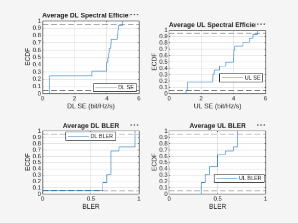
These results display the system KPIs, which include cell throughput, spectral efficiency, and empirical cumulative distribution function (ECDF) plots for both instantaneous cell throughput and average BLER. Use the ECDF plots to determine the proportion of slots in which throughput and BLER are less than or equal to specific values indicated on the x-axis.

Display the ECDF plots of average spectral efficiency and average BLER across all gNBs.

scenario.displayScenarioPlots(metricsVisualizer,numGNBs,numFrameSimulation)

Further Exploration

You can use this example to further explore these capabilities.

Evaluate Wideband SINR in the eMBB InH Scenario Against the 3GPP Reference Scenario

Refer to the CompareInHScenarioWith3GPPReferenceScenario.m script for details on the simulation scenario.

The assumptions and limitations of these simulations are:

RSRP-Based UE Attachment: UEs attached via RSRP measurements (path loss + shadow fading + antenna gain) per TR 38.901, with uniform dropping, and 20x oversampling, and random selection of exactly 10 UEs per gNB from attached candidates
Channel & Interference Modeling: h38901Channel with InterfererHasSmallScale=true enables small-scale fading for all 11 interfering gNBs per UE; deterministic seeding ensures reproducible realizations with aligned RNG between scenario builder and channel model
Performance Metrics: PDSCH SINR measured via PacketReceptionEnded listener with temporal averaging across slots (excluding 5ms stabilization); CDF compared against 3GPP RP-180524 reference; samples with SINR < -5 dB filtered due to no handover support
The simulation runs a full buffer traffic model, adopts resource allocation type 1 (RAT-1), and uses a round-robin scheduling algorithm.

The results also contain a comparison of the wideband SINR in the InH scenario with the 3GPP reference models, following the assumptions and specifications in RP-180524.

Evaluate Wideband SINR in the Dense-Urban Macro Scenario Against the 3GPP Reference Scenario

This section presents the Phase 1 calibration results for the Dense-Urban Macro-layer scenario at 4 GHz, following the evaluation assumptions in R1-1703534, Table 3. The layout includes 19 tri-sector sites, corresponding to 57 cells, with a 200 m inter-site distance and toroidal wraparound. Each gNB uses a 128-element cross-polarized array, represented by the configuration (8,8,2,1,1), and applies 1D vertical TXRU virtualization (K = 4) to generate 32 digital ports with a 12-degree electrical downtilt. Each UE uses a single cross-polarized omnidirectional element pair. The simulation drops ten UEs per cell with an 80% indoor and 20% outdoor distribution and selects the serving cell based on coupling loss.

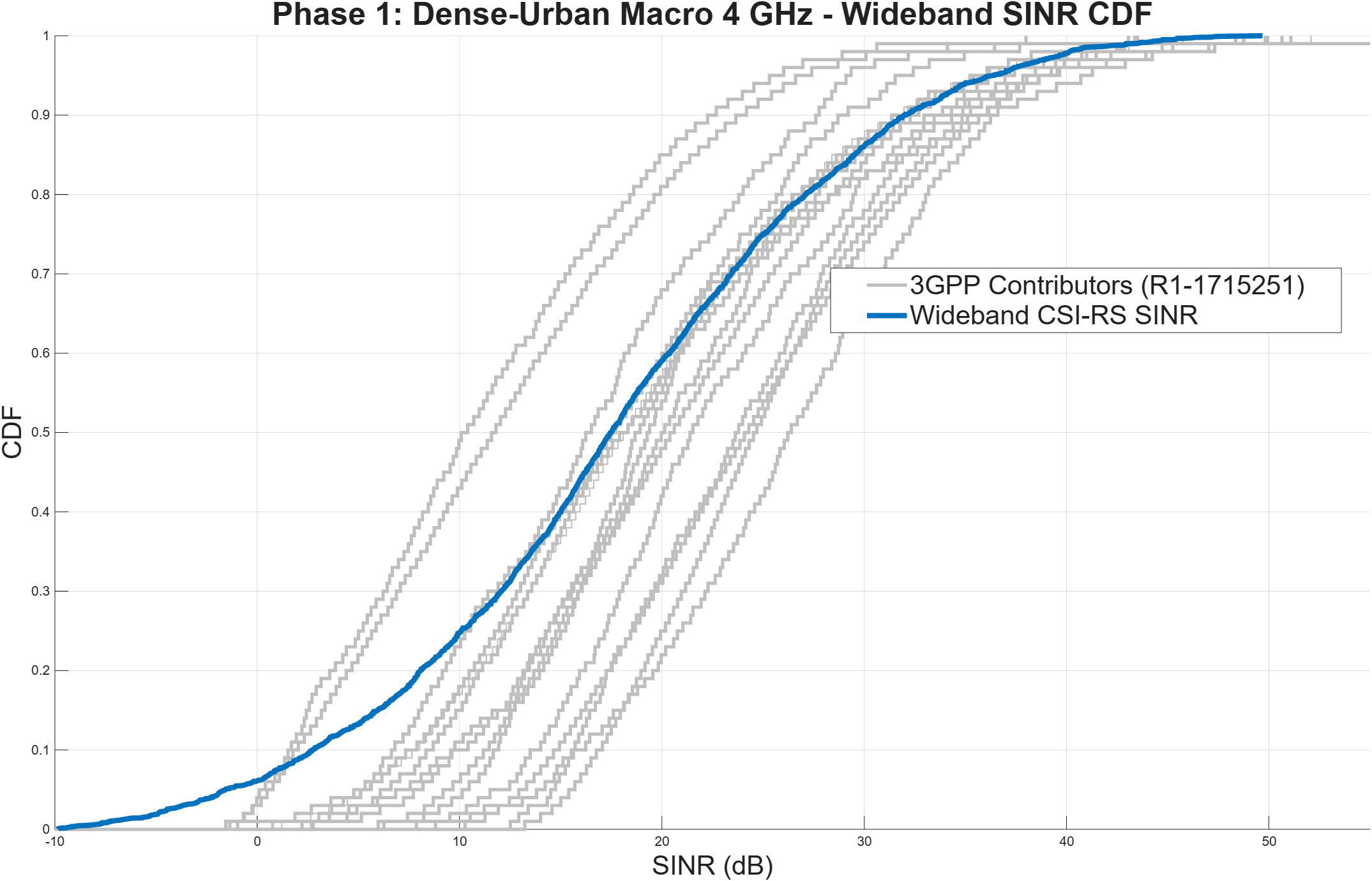
The simulation computes the wideband SINR. For the serving signal, it applies digital precoding across the 32-port codebook. For interference, it models each non-serving gNB using a single TXRU with one polarization and no digital precoding. The simulation runs five independent drops with approximately 570 UEs per drop, generating more than 2,800 SINR samples. The resulting CDF remains within the range of results reported by 3GPP contributors in R1-1715251.

The simulation uses these assumptions:

Panel Dimensions: The simulation uses a panel configuration of (2,8,2,1,1), corresponding to 32 antenna ports. It configures the codebook panel as [Ng, N1, N2] = [1, 8, 2], where N1 = 8 horizontal ports and N2 = 2 vertical ports per polarization. It applies TXRU virtualization using a 1D vertical DFT with K = 4 sub-elements per TXRU, expanding the panel to 128 antenna elements. It applies an electrical downtilt of 102°, corresponding to 12° below the horizon.
Precoding: The serving link uses a two-stage precoding architecture. It first performs analog beamforming through TXRU virtualization and then applies digital precoding. Interfering gNBs perform only analog beamforming. Each interfering gNB uses a single TXRU and a single polarization and does not apply digital precoding.
UE Receiver Assumptions: The simulation uses an MMSE-IRC receiver to obtain CSI measurements. However, it reports the wideband SINR as a pre-equalization metric and does not apply IRC combining in the SINR calculation.
UE Association: The simulation selects the serving cell based on coupling loss. When the analog beam codebook aligns with the TXRU tilt grid, this approach becomes equivalent to selecting the beam with the highest RSRP.
Wideband SINR Computation: The simulation computes the wideband SINR as the linear power ratio averaged across all resource blocks:

$S I N R = \frac{\frac{1}{K} {\sum_{k = 1}^{K} ‖ H_{k} W ‖}^{2}}{N + \frac{1}{K} \sum_{k = 1}^{K} \sum_{j} {‖ H_{j, k} w_{j} ‖}^{2}}$

Where,

$K$ is the number of resource blocks.

$H_{k}$ is the serving-channel matrix on resource block $k$ .

$W$ is the serving precoder.

$H_{j, k}$ is the interference-channel matrix from the $j^{t h}$ non-serving gNB on resource block $k$ .

$w_{j}$ is the single-TXRU interference weight for the $j^{t h}$ non-serving gNB.

$N$ is the noise power.

Key Findings from Wideband SINR Evaluation

CDF Comparison with the 3GPP Reference: The simulated SINR CDF closely matches the 3GPP reference results in the median and upper-percentile regions. Applying the TR 38.901 outdoor-to-indoor penetration model to 80% of UEs, which represent indoor users, extends the lower tail below most contributor results.
Impact of Very Low SINR Samples: SINR values below −10 dB account for only 0.6% of all samples. Excluding these samples produces a negligible change in the overall SINR distribution.

Analyze the Impact of Link Adaptation, Channel, and Antenna Configuration on KPIs

You can specify different antenna configurations, LA parameters, and transmit power and analyze their impact on the system KPIs such as the throughput, spectral efficiency and BLER.
You can also adjust the parameters such as "OfficeType" and "InterfererHasSmallScale" in the channel configuration to observe their impact on the system KPIs. When you enable the "InterfererHasSmallScale" parameter, the simulation includes small-scale fading, providing a more accurate representation of interference. However, if your priority is computational efficiency in the simulation, disabling this feature can significantly increase simulation speed.

Supporting Functions

The example uses these helper objects and functions:

helperNRMetricsVisualizer — Implements metrics visualization functionality
h3GPPReferenceScenarios — Generates InH scenario
h38901Channel — Implements 3GPP TR 38.901 channel model
h38901Scenario — Implements 3GPP TR 38.901 system-level scenario builder
hNRKPIManager — Implements functionality for calculating key performance indicators

References

[1] 3GPP TR 38.913. “Study on Scenarios and Requirements for Next Generation Access Technologies.” Release 17. 3rd Generation Partnership Project; Technical Specification Group Radio Access Network.

[2] Huawei, Summary of Calibration Results for IMT-2020 Self Evaluation, 3GPP TSG RAN Meeting 79, RP-180524, 2018.