Deploy Industrial Cooling Fan Anomaly Detection Algorithm as Microservice

This example uses:

This example details the process of transforming the Industrial Cooling Fan Anomaly Detection Algorithm Development for Deployment to a Microservice Docker Image (Predictive Maintenance Toolbox) into a Docker® microservice. The primary goal is to provide an HTTP/HTTPS endpoint for accessing the algorithm, which is essential for integrating into a predictive maintenance framework.

The process begins by packaging the support vector machine-based anomaly detection algorithm, developed using the Predictive Maintenance Toolbox™ in MATLAB®, into a deployable archive. This archive encompasses the trained model capable of identifying anomalies in load, fan mechanics, and power consumption of an industrial cooling fan. Following this, a Docker image is created, incorporating the deployable archive along with a minimal MATLAB® Runtime package.

Once the Docker image is prepared, it can be deployed within a Docker environment. You can use the MATLAB Production Server™ client APIs to make calls to the microservice.

Prerequisites

Verify that you have trained anomaly detection model anomalyDetectionModelSVM.mat file that contains the anomaly detection model and the validationEnsemble.mat file containing the test data.
Verify that you have MATLAB Compiler SDK installed on the development machine.
Verify that you have Docker installed and configured on the development machine by typing [~,msg] = system('docker version') in a MATLAB command window. Note: If you are using WSL, use the command [~,msg] = system('wsl docker version') instead.If you do not have Docker installed, follow the instructions on the Docker website to install and set up Docker. docs.docker.com/engine/install/
To build microservice images on Windows, you must install either Docker Desktop or Docker on Windows Subsystem for Linux v2 (WSL2). To install Docker Desktop, see https://docs.docker.com/desktop/install/windows-install/
For instructions on how to install Docker on WSL2, see https://www.mathworks.com/matlabcentral/answers/1758410-how-do-i-install-docker-on-wsl2.
Verify that you have the MATLAB Runtime installer for Linux on your machine. You can download the installer from the MathWorks website: https://www.mathworks.com/products/compiler/matlab-runtime.html

Create MATLAB Function

Create a MATLAB function named detectCoolingFanAnomaly that is designed to process industrial cooling fan data for reliable anomaly detection. The function takes a matrix or timetable x containing cooling fan measurements, and an optional categorical array y with true anomalies, to form a data ensemble and calculate diagnostic features. After loading a pre-trained SVM model from anomalyDetectionModelSVM.mat, it predicts anomalies and returns predictedAnomalies and, if provided, trueAnomalies.

function [predictedAnomalies, trueAnomalies] = detectCoolingFanAnomaly(x, y)

% Load model
model=load('anomalyDetectionModelSVM.mat');
anomalyDetectionModel=model.m;

windowSize = size(x, 1);
ensembleTable1 = generateEnsembleTable(x,y(:,1),windowSize);
ensembleTable2 = generateEnsembleTable(x,y(:,2),windowSize);
ensembleTable3 = generateEnsembleTable(x,y(:,3),windowSize);

featureTable1 = diagnosticFeatures_streaming(ensembleTable1);
featureTable2 = diagnosticFeatures_streaming(ensembleTable2);
featureTable3 = diagnosticFeatures_streaming(ensembleTable3);

% Predict
results1 = anomalyDetectionModel.m1.predict(featureTable1);
results2 = anomalyDetectionModel.m2.predict(featureTable2);
results3 = anomalyDetectionModel.m3.predict(featureTable3);

predictedAnomalies = [results1, results2, results3];
trueAnomalies = [ensembleTable1.Anomaly, ensembleTable2.Anomaly, ensembleTable3.Anomaly];
end

Supporting Files

IndexIterator.m - The IndexIterator class provides a mechanism to iterate over a range of indices in configurable windows or frames. It allows for sequential access to subsets of indices, with control over the window size and step size between indices.

generateEnsembleTable.m - The generateEnsembleTable function segments a matrix of signal data x into windows of a specified size ws and associates each segment with a binary label indicating if it's an anomaly based on the sum of labels y. The result is a table with each row containing a signal window and its corresponding anomaly label.

diagnosticFeatures_streaming.m - The diagnosticFeatures_streaming function computes various time series features from multiple signals within an input timetable, including autoregressive model coefficients, frequencies, AIC, mean, RMS, ACF, and PACF. The calculated features are then organized into a table, which is returned as the output for further analysis or modeling.

anomalyDetectionModelSVM.mat - Anomaly detection model.

validationEnsemble.mat - Validation data.

Test the function from the MATLAB command line:

load validationEnsemble
validationData = validationEnsemble.readall;
anomaly_data_validation = vertcat(validationData.Anomalies{1}.Data);

yValidationAnomaly1=logical(anomaly_data_validation(:,1));
yValidationAnomaly2=logical(anomaly_data_validation(:,2));
yValidationAnomaly3=logical(anomaly_data_validation(:,3));

sensorDataValidation = vertcat(validationData.Signals{:}.Data);

windowSize = 2000;
ii = IndexIterator(1, size(sensorDataValidation,1), windowSize);
predictedLabel = nan(floor(size(sensorDataValidation,1)/windowSize), 3);
trueLabel = nan(floor(size(sensorDataValidation,1)/windowSize), 3);
counter = 1;
while ~ii.EndofRangeFlag
    frame = ii.nextFrameIndex;
    [predictedLabel(counter, :), trueLabel(counter, :)] = ...
    detectCoolingFanAnomaly(sensorDataValidation(frame(1):frame(2), 1:3), ...
    anomaly_data_validation(frame(1):frame(2), 1:3));
    counter = counter+1;
end
reset(ii);

tiledlayout(1,3);
nexttile; confusionchart(trueLabel(:,1), predictedLabel(:,1));
nexttile; confusionchart(trueLabel(:,2), predictedLabel(:,2));
nexttile; confusionchart(trueLabel(:,3), predictedLabel(:,3));

Create Deployable Archive

Package the detectCoolingFanAnomaly function into a deployable archive using the compiler.build.productionServerArchive function.

buildResults = compiler.build.productionServerArchive('detectCoolingFanAnomaly.m', ...
    ArchiveName='coolingFanAnomaly', ...
    Verbose=true)

The buildResults object contains information on the build type, generated files, included support packages, and build options.

Once the build is complete, the function creates a folder named coolingFanAnomalyproductionServerArchive in your current directory to store the deployable archive.

Package Archive into Microservice Docker Image

Build the microservice Docker image using the buildResults object that you created. You can specify additional options in the compiler.build command by using name-value arguments. For details, see compiler.package.microserviceDockerImage.

compiler.package.microserviceDockerImage(buildResults, ...
    ImageName='detect-cooling-fan-microservice', ...
    DockerContext=fullfile(pwd,'microserviceDockerContext'), ...
    VerbosityLevel='concise');

The function generates the following files within a folder named microserviceDockerContext in your current working directory:

applicationFilesForMATLABCompiler/coolingFanAnomaly.ctf — Deployable archive file.
Dockerfile — Docker file that specifies Docker run-time options.
GettingStarted.txt — Text file that contains deployment information.

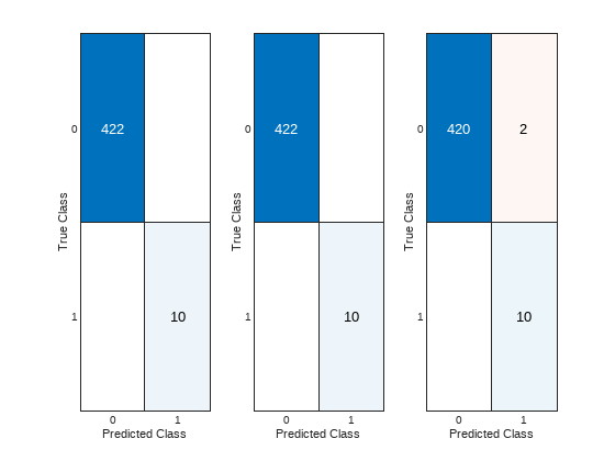
Test Docker Image

Once the Docker container is initialized, verify the enclosed algorithm by reusing data from validationEnsemble. Follow the established procedure: divide the data into windows, each containing 2000 samples, and use these to construct the message body for an HTTP POST request. The response from this request includes the predicted anomaly status, which is then compared against the true labels to assess the algorithm's accuracy.

In a system command window, verify that your detect-cooling-fan-microservice image is in your list of Docker images.

docker images

REPOSITORY                                       TAG                      IMAGE ID       CREATED         SIZE
detect-cooling-fan-microservice                  latest                   af24e3fe610c   2 days ago      3.94GB

Run the detectCoolingFan-microservice image from the system command prompt.

docker run --rm -p 9900:9910 detectCoolingFan-microservice -l trace &

Port 9910 is the default port exposed by the microservice within the Docker container. You can map it to any available port on your host machine. For this example, it is mapped to port 9900.

You can specify additional options in the Docker command. For a complete list of options, see Microservice Command Arguments.

Once the microservice container is running in Docker, you can check the status of the service by going to the following URL in a web browser: http://hostname:9900/api/health

If the service is ready to receive requests, you see the following message: "status: ok"

Send Request from MATLAB

import matlab.net.http.*
import matlab.net.http.field.*
data = matlab.net.http.MessageBody();

windowSize = 2000;
ii = IndexIterator(1, size(sensorDataValidation, 1), windowSize);
predictedLabel = nan(floor(size(sensorDataValidation,1)/windowSize), 3);
trueLabel = nan(floor(size(sensorDataValidation,1)/windowSize), 3);
counter = 1;

while ~ii.EndofRangeFlag
    frame = ii.nextFrameIndex;

    rhs = {sensorDataValidation(frame(1):frame(2), :), anomaly_data_validation(frame(1):frame(2), :)};
    data.Payload = mps.json.encoderequest(rhs, 'Nargout', 2, 'OutputFormat', 'large');
    request = RequestMessage('POST', ...
        [HeaderField('Content-Type', 'application/json')], ...
        data);

    response = request.send('http://localhost:9900/coolingFanAnomaly/detectCoolingFanAnomaly');
    predictedLabel(counter, :) = response.Body.Data.lhs(1).mwdata';
    trueLabel(counter, :) = response.Body.Data.lhs(2).mwdata';
    counter = counter+1;
end
reset(ii);
 
figure;
tiledlayout(1,3)
nexttile; confusionchart(trueLabel(1:250,1), predictedLabel(1:250,1));
nexttile; confusionchart(trueLabel(1:250,2), predictedLabel(1:250,2));
nexttile; confusionchart(trueLabel(1:250,3), predictedLabel(1:250,3));

The anomaly detection algorithm in the docker container can now be integrated into existing IT/OT infrastructure and managed with Kubernetes for high availability and to manage large volumes of requests. The docker image can be easily shared with other members for testing the algorithm and also for integration into other systems.

Note: This microservice is designed for universal accessibility and can be interfaced with using any programming language, command line tools like cURL, or through MATLAB Production Server client APIs. To ensure seamless interaction and accurate processing, it is crucial to format the validation data appropriately for the specific language or tool being used. While this documentation predominantly illustrates examples using MATLAB for ease of explanation, the guidelines for data formatting and interacting with the service are relevant and can be adapted to various programming contexts.