timeoptions
Create list of time plot options
Description
Use the timeoptions command to create a
TimeOptions object to customize time plot appearance. Use this object to
customize the appearance of a time plot created using impulseplot, initialplot, lsimplot, or stepplot and override the plot preferences for the MATLAB® session in which you create the time plot.
The options you specify for a TimeOptions object correspond to properties
of the ImpulsePlot, InitialPlot,
LSimPlot or StepPlot chart object.
Creation
Description
plotoptions = timeoptions
plotoptions = timeoptions("cstprefs")
Properties
Response
Option to normalize plot, specified as either 'on' or
'off'.
This option corresponds to the Normalize property of the
chart object.
Settling time threshold, specified as a positive scalar less than
1.
This option is ignored by lsimplot.
This option corresponds to the
Characteristics.ConfidenceRegion.SettlingTime.Threshold
property of the chart object.
Rise time limits between the values of 0 and
1, specified as a two-element vector of the form
[min,max].
This option is supported only for stepplot.
This option corresponds to the
Characteristics.RiseTime.Limits property of the chart
object.
Number of standard deviations to use to plot the confidence region, specified as a scalar. This option is applicable to identified models only.
This option is supported only for stepplot and
impulseplot.
This option corresponds to the
Characteristics.ConfidenceRegion.NumberOfStandardDeviations
property of the chart object.
Dependencies
This option is supported only for identified models, which require System Identification Toolbox software.
Units
Time units, specified as one of the following values:
'nanoseconds''microseconds''milliseconds''seconds''minutes''hours''days''weeks''months''years'
You can also specify 'auto' which uses time units specified in
the TimeUnit property of the input system. For multiple systems
with different time units, the units of the first system are used.
This option corresponds to the TimeUnit property of the chart
object.
Inputs and Outputs
Grouping of input-output (I/O) pairs, specified as one of the following:
'none'— Do not group inputs or outputs.'inputs'— Group only inputs.'outputs'— Group only outputs.'all'— Group all input-output pairs.
lsimplot and initialplot support only
the 'none' and 'all' values.
This option corresponds to the IOGrouping property of the
chart object.
Input label style, specified as a structure with the following fields:
FontSize— Font size, specified as a scalar value greater than zero in point units. The default font size depends on the specific operating system and locale. One point equals1/72inch.FontWeight— Character thickness, specified as'Normal'or'bold'. MATLAB uses theFontWeightproperty to select a font from those available on your system. Not all fonts have a bold weight. Therefore, specifying a bold font weight can still result in the normal font weight.FontAngle— Character slant, specified as'Normal'or'italic'. Not all fonts have both font styles. Therefore, the italic font might look the same as the normal font.Color— Text color, specified as an RGB triplet. The default color is dark gray with the RGB triplet[0.4,0.4,0.4].Interpreter— Text interpreter, specified as one of these values:'tex'— Interpret characters using a subset of TeX markup. This is the default value ofInterpreter.'latex'— Interpret characters using LaTeX markup.'none'— Display literal characters.
This property is ignored by lsimplot and
initialplot.
This option corresponds to the InputLabels property of the
chart object.
Output label style, specified as a structure with the following fields:
FontSize— Font size, specified as a scalar value greater than zero in point units. The default font size depends on the specific operating system and locale. One point equals1/72inch.FontWeight— Character thickness, specified as'Normal'or'bold'. MATLAB uses theFontWeightproperty to select a font from those available on your system. Not all fonts have a bold weight. Therefore, specifying a bold font weight can still result in the normal font weight.FontAngle— Character slant, specified as'Normal'or ''italic'. Not all fonts have both font styles. Therefore, the italic font might look the same as the normal font.Color— Text color, specified as an RGB triplet. The default color is dark gray with the RGB triplet[0.4,0.4,0.4].Interpreter— Text interpreter, specified as one of these values:'tex'— Interpret characters using a subset of TeX markup. This is the default value ofInterpreter.'latex'— Interpret characters using LaTeX markup.'none'— Display literal characters.
This option corresponds to the OutputLabels property of the
chart object.
Option to display inputs, specified as {'on'},
{'off'}, or a cell array with multiple elements.
This property is ignored by lsimplot and
initialplot.
This option corresponds to the InputVisible property of the
chart object.
Option to display outputs, specified as {'on'},
{'off'}, or a cell array with multiple elements.
This option corresponds to the OutputVisible property of the
chart object.
Title and Axis Labels
Title text and style, specified as a structure with the following fields:
String— Label text, specified as a character vector. By default, the plot is titled 'Bode Diagram'.FontSize— Font size, specified as a scalar value greater than zero in point units. The default font size depends on the specific operating system and locale. One point equals1/72inch.FontWeight— Character thickness, specified as'Normal'or'bold'. MATLAB uses theFontWeightproperty to select a font from those available on your system. Not all fonts have a bold weight. Therefore, specifying a bold font weight can still result in the normal font weight.FontAngle— Character slant, specified as'Normal'or'italic'. Not all fonts have both font styles. Therefore, the italic font might look the same as the normal font.Color— Text color, specified as an RGB triplet. The default color is black specified by the RGB triplet[0,0,0].Interpreter— Text interpreter, specified as one of these values:'tex'— Interpret characters using a subset of TeX markup. This is the default value ofInterpreter.'latex'— Interpret characters using LaTeX markup.'none'— Display literal characters.
This option corresponds to the Title property of the chart object.
X-axis label text and style, specified as a structure with the following fields:
String— Label text, specified as a character vector. By default, the axis is titled based on the frequency unitsFreqUnits.FontSize— Font size, specified as a scalar value greater than zero in point units. The default font size depends on the specific operating system and locale. One point equals1/72inch.FontWeight— Character thickness, specified as'Normal'or'bold'. MATLAB uses theFontWeightproperty to select a font from those available on your system. Not all fonts have a bold weight. Therefore, specifying a bold font weight can still result in the normal font weight.FontAngle— Character slant, specified as'Normal'or'italic'. Not all fonts have both font styles. Therefore, the italic font might look the same as the normal font.Color— Text color, specified as an RGB triplet. The default color is black specified by the RGB triplet[0,0,0].Interpreter— Text interpreter, specified as one of these values:'tex'— Interpret characters using a subset of TeX markup. This is the default value ofInterpreter.'latex'— Interpret characters using LaTeX markup.'none'— Display literal characters.
This option corresponds to the XLabel property of the chart object.
Y-axis label text and style, specified as a structure with the following fields:
String— Label text, specified as a cell array of character vectors. By default, the axis label is a 1x2 cell array with 'Magnitude' and 'Phase'.FontSize— Font size, specified as a scalar value greater than zero in point units. The default font size depends on the specific operating system and locale. One point equals1/72inch.FontWeight— Character thickness, specified as'Normal'or'bold'. MATLAB uses theFontWeightproperty to select a font from those available on your system. Not all fonts have a bold weight. Therefore, specifying a bold font weight can still result in the normal font weight.FontAngle— Character slant, specified as'Normal'or'italic'. Not all fonts have both font styles. Therefore, the italic font might look the same as the normal font.Color— Text color, specified as an RGB triplet. The default color is black specified by the RGB triplet[0,0,0].Interpreter— Text interpreter, specified as one of these values:'tex'— Interpret characters using a subset of TeX markup. This is the default value ofInterpreter.'latex'— Interpret characters using LaTeX markup.'none'— Display literal characters.
This option corresponds to the YLabel property of the chart object.
Tick label style, specified as a structure with the following fields:
FontSize— Font size, specified as a scalar value greater than zero in point units. The default font size depends on the specific operating system and locale. One point equals1/72inch.FontWeight— Character thickness, specified as'Normal'or'bold'. MATLAB uses theFontWeightproperty to select a font from those available on your system. Not all fonts have a bold weight. Therefore, specifying a bold font weight can still result in the normal font weight.FontAngle— Character slant, specified as'Normal'or'italic'. Not all fonts have both font styles. Therefore, the italic font might look the same as the normal font.Color— Text color, specified as an RGB triplet. The default color is black specified by the RGB triplet[0,0,0].
Grid
Toggle grid display on the plot, specified as either 'off' or 'on'.
This option corresponds to the GridVisible property of the chart object.
Color of the grid lines, specified as an RGB triplet. The default color is light gray
specified by the RGB triplet [0.15 0.15 0.15].
Axis Limits
X-axis limit selection mode, specified as one of the following values:
'auto'— Enable automatic limit selection, which is based on the total span of the plotted data.'manual'— Manually specify the axis limits. To specify the axis limits, set theXLimoption.
This option corresponds to the XLimitsMode property of the chart object.
Selection mode for the y-axis limits, specified as one of these values:
'auto'— Enable automatic limit selection, which is based on the total span of the plotted data.'manual'— Manually specify the axis limits. To specify the axis limits, set theYLimoption.
This option corresponds to the YLimitsMode property of the chart object.
X-axis limits, specified as a cell array of two-element vector of the form [min,max].
This option corresponds to the XLimits property of the chart object.
Y-axis limits, specified as a cell array of two-element vector of the form [min,max].
This option corresponds to the YLimits property of the chart object.
Object Functions
impulseplot | Plot impulse response of dynamic system |
initialplot | Plot initial condition response of dynamic system |
lsimplot | Plot simulated time response of dynamic system to arbitrary inputs |
stepplot | Plot step response of dynamic system |
Examples
Create a default time options set.
opt = timeoptions;
Enable plotting of normalized responses.
opt.Normalize = 'on';Plot the step response of two transfer function models using the specified options.
sys1 = tf(10,[1,1]);
sys2 = tf(5,[1,5]);
stepplot(sys1,sys2,opt);
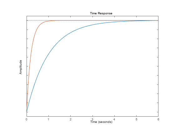
The plot shows the normalized step response for the two transfer function models.
For this example, use the plot handle to change the time units to minutes and turn on the grid.
Generate a random state-space model with 5 states and create the step response plot with chart object sp.
rng("default")
sys = rss(5);
sp = stepplot(sys);
Change the time units to minutes and turn on the grid. To do so, edit properties of the chart object.
sp.TimeUnit = "minutes";
grid on;

The step plot automatically updates when you modify the chart object.
Alternatively, you can also use the timeoptions command to specify the required plot options. First, create an options set based on the toolbox preferences.
plotoptions = timeoptions("cstprefs");Change properties of the options set by setting the time units to minutes and enabling the grid.
plotoptions.TimeUnits = 'minutes';
plotoptions.Grid = "on";
stepplot(sys,plotoptions);

Depending on your own toolbox preferences, the plot you obtain might look different from this plot. Only the properties that you set explicitly, in this example TimeUnits and Grid, override the toolbox preferences.
For this example, examine the step response of the following zero-pole-gain model and limit the step plot to tFinal = 15 s. Use 15-point blue text for the title. This plot should look the same, regardless of the preferences of the MATLAB session in which it is generated.
sys = zpk(-1,[-0.2+3j,-0.2-3j],1)*tf([1 1],[1 0.05]);
tFinal = 15;
First, create a default options set using timeoptions.
plotoptions = timeoptions;
Next change the required properties of the options set plotoptions.
plotoptions.Title.FontSize = 15;
plotoptions.Title.Color = [0 0 1];
Now, create the step response plot using the options set plotoptions.
h = stepplot(sys,tFinal,plotoptions);

Because plotoptions begins with a fixed set of options, the plot result is independent of the toolbox preferences of the MATLAB session.
By default, lsimplot simulates the model assuming all states are zero at the start of the simulation. When simulating the response of a state-space model, use the optional x0 input argument to specify nonzero initial state values. Consider the following two-state SISO state-space model.
A = [-1.5 -3;
      3   -1];
B = [1.3; 0];
C = [1.15 2.3];
D = 0;
sys = ss(A,B,C,D);
Suppose that you want to allow the system to evolve from a known set of initial states with no input for 2 s, and then apply a unit step change. Specify the vector x0 of initial state values, and create the input vector.
x0 = [-0.2 0.3];
t = 0:0.05:8;
u = zeros(length(t),1);
u(t>=2) = 1;
First, create a default options set using timeoptions.
plotoptions = timeoptions;
Next change the required properties of the options set plotoptions and plot the simulated response with the zero order hold option.
plotoptions.Title.FontSize = 15;
plotoptions.Title.Color = [0 0 1];
plotoptions.Grid = 'on';
h = lsimplot(sys,u,t,x0,plotoptions,'zoh');
hold on
title('Simulated Time Response with Initial Conditions')
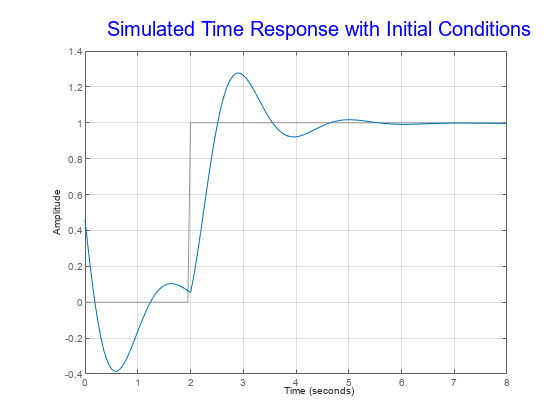
The first half of the plot shows the free evolution of the system from the initial state values [-0.2 0.3]. At t = 2 there is a step change to the input, and the plot shows the system response to this new signal beginning from the state values at that time. Because plotoptions begins with a fixed set of options, the plot result is independent of the toolbox preferences of the MATLAB session.
For this example, change time units to minutes and turn the grid on for the simulated response plot. Consider the following transfer function.
sys = tf(3,[1 2 3]);
To compute the response of this system to an arbitrary input signal, provide lsimplot with a vector of the times t at which you want to compute the response and a vector u containing the corresponding signal values. For instance, plot the system response to a ramping step signal that starts at 0 at time t = 0, ramps from 0 at t = 1 to 1 at t = 2, and then holds steady at 1. Define t and compute the values of u.
t = 0:0.04:8;
u = max(0,min(t-1,1));
Use lsimplot plot the system response to the signal with chart object lp.
lp = lsimplot(sys,u,t);
grid on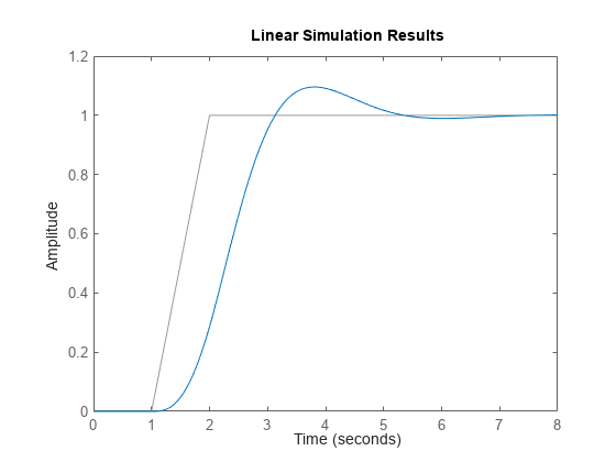
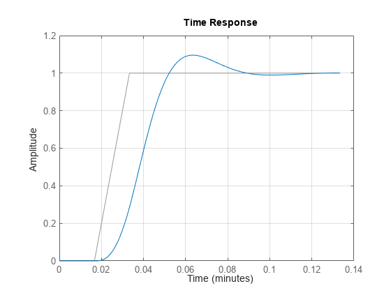
The plot shows the applied input (u,t) in gray and the system response in blue.
Modify the chart object to change the time units to minutes.
lp.TimeUnit = "minutes";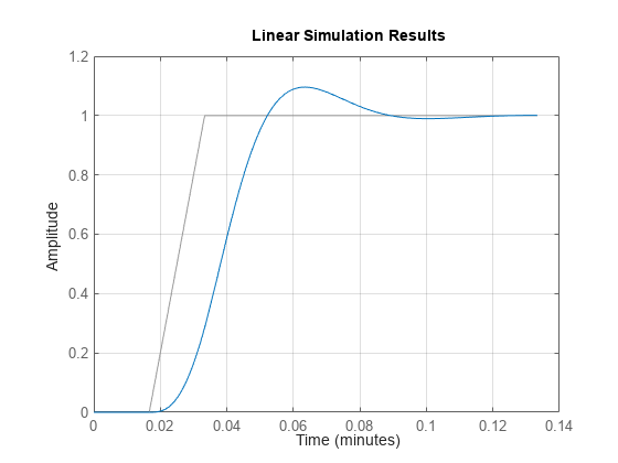
The plot automatically updates when you modify the chart object.
Alternatively, you can also use the timeoptions command to specify the required plot options. First, create an options set based on the toolbox preferences.
plotoptions = timeoptions('cstprefs');Change properties of the options set by setting the time units to minutes and enabling the grid.
plotoptions.TimeUnits = 'minutes';
plotoptions.Grid = 'on';
lsimplot(sys,u,t,plotoptions);
Version History
Introduced in R2008a
See Also
MATLAB Command
You clicked a link that corresponds to this MATLAB command:
Run the command by entering it in the MATLAB Command Window. Web browsers do not support MATLAB commands.
Select a Web Site
Choose a web site to get translated content where available and see local events and offers. Based on your location, we recommend that you select: .
You can also select a web site from the following list
How to Get Best Site Performance
Select the China site (in Chinese or English) for best site performance. Other MathWorks country sites are not optimized for visits from your location.
Americas
- América Latina (Español)
- Canada (English)
- United States (English)
Europe
- Belgium (English)
- Denmark (English)
- Deutschland (Deutsch)
- España (Español)
- Finland (English)
- France (Français)
- Ireland (English)
- Italia (Italiano)
- Luxembourg (English)
- Netherlands (English)
- Norway (English)
- Österreich (Deutsch)
- Portugal (English)
- Sweden (English)
- Switzerland
- United Kingdom (English)