Yaw Damper Design for 747 Jet Aircraft

This example shows the design of a YAW DAMPER for a 747® aircraft using the classical control design features in Control System Toolbox™.

The example uses a simplified trim model of the aircraft during cruise flight. This model has two inputs (runner and aileron deflections) and the following four states:

All angles and angular velocities are in radians and radians/sec, respectively,

Specify the A, B, C, and D matrices of the trim model and create state-space model sys.

A = [-0.0558 -0.9968  0.0802 0.0415;
       0.598  -0.115 -0.0318      0;
       -3.05   0.388 -0.4650      0;
           0  0.0805       1      0];

B = [ 0.00729       0;
       -0.475 0.00775;
        0.153   0.143;
            0       0];

C = [0 1 0 0;
     0 0 0 1];

D = [0 0;
     0 0];

sys = ss(A,B,C,D);

Label the inputs, outputs, and states.

sys.InputName = ["rudder" "aileron"];
sys.OutputName = ["yaw rate" "bank angle"];
sys.StateName = ["beta" "yaw" "roll" "phi"];

This model has a pair of lightly damped poles that correspond to the Dutch roll mode. View the poles using a pole-zero plot and sisplay the grid with damping and natural frequency values.

pzplot(sys)
grid on

Your goal for this example is to design a compensator that increases the damping of these two poles.

To determine possible control strategies, start with some open-loop analysis. The impulse responseis highly oscillatory, which confirms the presence of lightly damped modes.

ip = impulseplot(sys);

Inspect the response over a shorter time frame of 20 seconds.

ip = impulseplot(sys,20);

View the response from the aileron deflection to the bank angle. To show only this plot, right-click the plot and select I/O Selector. Then, in the I/O Selector dialog box, select the entry in the aileron column and bank angle row.

Alternatively, hide the display for the first input and the first output by modifying chart object ip.

ip.InputVisible(1) = "off";
ip.OutputVisible(1) = "off";

This plot shows the aircraft oscillating around a nonzero bank angle, which means that the aircraft turns in response to an aileron impulse.

Typically, yaw dampers are designed using yaw rate as the sensed output and rudder as the input. Extract this model from the original system and view its frequency response.

sys11 = sys("yaw","rudder");
bodeplot(sys11);

This plot shows that the rudder has a lot of authority around the lightly damped Dutch roll mode (1 rad/s).

A reasonable design objective is to provide a damping ratio $\zeta$ > 0.35, with natural frequency $w_n$ < 1.0 rad/s. The simplest compensator is a gain.

Use the root locus technique to select an adequate feedback gain value.

rlocusplot(sys11);

This plot assumes negative feedback and has much of the root locus is in the right-half plane.

Switch to positive feedback, which places the root locus in the left-hand plane

rlocusplot(-sys11)

To view gain and damping values, click the blue curve. The best achievable closed-loop damping is about 0.45 for a gain of $k$ = 2.85.

Close the SISO feedback loop and view the impulse response. By default, the feedback function assumes negative feedback, therefore specify the feedback gain as –$k$.

k = 2.85;
cl11 = feedback(sys11,-k);

impulseplot(sys11,"b--",cl11,"r")
legend("open-loop","closed-loop",Location="SouthEast");

The closed-loop response looks good..

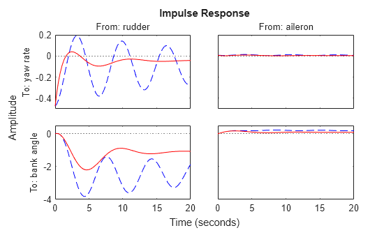
To view the response from the aileron, close the loop around the full MIMO model. The feedback loop involves input 1 and output 1 of the plant.

cloop = feedback(sys,-k,1,1);
impulseplot(sys,"b--",cloop,"r",20)

The yaw rate response is now well-damped.

However, when moving the aileron, the system no longer continues to bank like a normal aircraft, as shown in the following plot.

impulseplot(cloop("bank angle","aileron"),"r",18)

This result is due to an over-stabilized spiral mode. The spiral mode is typically a very slow mode that allows the aircraft to bank and turn without constant aileron input. Pilots are used to this behavior and will not like a design that does not fly normally.

To prevent the spiral mode from moving farther into the left-half plane when you close the loop, you can a washout filter as shown in this equation.

Using Control System Designer, you can graphically tune the parameters $k$ and $a$ to find the best combination. In this example, use $a$ = 0.2, which corresponds to a time constant of 5 seconds.

Create the washout filter for $a$ = 0.2 and $k$ = 1.

H = zpk(0,-0.2,1);

Connect the washout filter in series with the design model and use the root locus to determine the filter gain k.

oloop = H * (-sys11);
rlocusplot(oloop);
grid

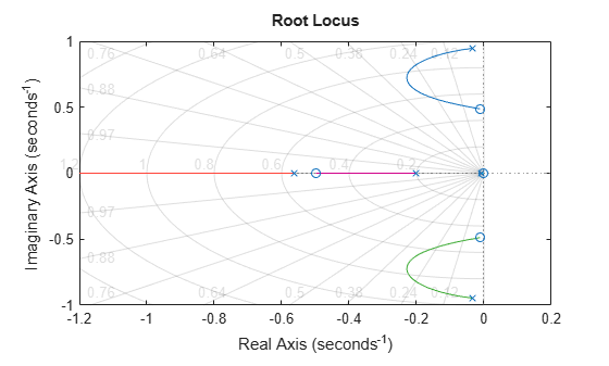
The best damping is now about $\zeta$ = 0.305 for $k$ = 2.34. Modify the filter gain, close the loop with the MIMO model, and check the impulse response.

k = 2.34;
wof = -k * H;
cloop = feedback(sys,wof,1,1);
impulseplot(sys,"b--",cloop,"r",20)

The washout filter has also restored the normal bank-and-turn behavior as seen by looking at the impulse response from aileron to bank angle.

impulseplot(sys(2,2),"b--",cloop(2,2),"r",20)
legend("open-loop","closed-loop",Location="southeast");

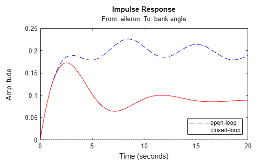
Although it does not quite meet the requirements, this design substantially increases the damping while allowing the pilot to fly the aircraft normally.

See Also

Functions

• rlocusplot | impulseplot | bodeplot

Apps

• Control System Designer

Topics

• Root Locus Design