Fit Power Series Models
About Power Series Models
The toolbox provides a one-term and a two-term power series model as given by
Power series models describe a variety of data. For example, the rate at which reactants are consumed in a chemical reaction is generally proportional to the concentration of the reactant raised to some power.
Fit Power Series Models Interactively
Open the Curve Fitter app by entering
curveFitterat the MATLAB® command line. Alternatively, on the Apps tab, in the Math, Statistics and Optimization group, click Curve Fitter.In the Curve Fitter app, select curve data. On the Curve Fitter tab, in the Data section, click Select Data. In the Select Fitting Data dialog box, select X data and Y data, or just Y data against an index.
Click the arrow in the Fit Type section to open the gallery, and click Power in the Regression Models group.

You can specify the following options in the Fit Options pane:
Specify the number of terms as
1or2. Look in the Results pane to see the model terms, values of the coefficients, and goodness-of-fit statistics.Optionally, in the Advanced Options section, specify coefficient starting values and constraint bounds, or change algorithm settings. The app calculates optimized start points for Power fits, based on the data set. You can override the start points and specify your own values in the Fit Options pane.
For more information on the settings, see Coefficient Constraints: Specify Bounds and Optimized Start Points.
Fit Power Series Models Using the fit Function
This example shows how to use the fit function to fit power series models to data.
The power series library model is an input argument to the fit and fittype functions. Specify the model type 'power1' or 'power2'.
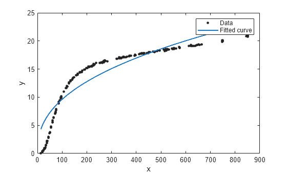
Fit a Single-Term Power Series Model
load hahn1;
f = fit(temp,thermex,'power1')
f =
     General model Power1:
     f(x) = a*x^b
     Coefficients (with 95% confidence bounds):
       a =        1.46  (1.224, 1.695)
       b =      0.4094  (0.3825, 0.4363)
plot(f,temp,thermex)
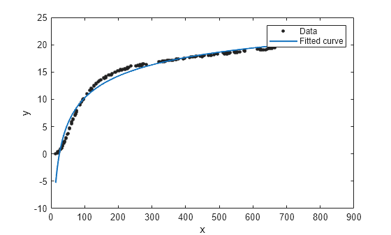
Fit a Two-Term Power Series Model
f = fit(temp,thermex,'power2')f =
General model Power2:
f(x) = a*x^b+c
Coefficients (with 95% confidence bounds):
a = -78.61 (-80.74, -76.48)
b = -0.2349 (-0.271, -0.1989)
c = 36.9 (33.09, 40.71)
plot(f,temp,thermex)
See Also
Apps
Functions
fit|fittype|fitoptions