Estimate the Transfer Function of a Circuit with ADALM1000

R2026b

This example uses:

Data Acquisition Toolbox Data Acquisition Toolbox
Data Acquisition Toolbox Support Package for Analog Devices ADALM1000 Hardware Data Acquisition Toolbox Support Package for Analog Devices ADALM1000 Hardware
Signal Processing Toolbox Signal Processing Toolbox

This example shows how to use MATLAB® to connect to an ADALM1000 source-measurement unit, configure it to generate an arbitrary signal, make live measurements, and use the measurements to calculate the transfer function of the connected circuit.

Introduction

In this example you have an R-C circuit consisting of a 1 k $Ω$ resistor in series with a 0.1 $μ$ F capacitor. The R-C circuit is attached to the ADALM1000 device with Channel A of the device providing the voltage stimulus consisting of a chirp signal. The output of Channel A is connected to the resistor, and the ground is connected to the capacitor. Channel B of the device is used to measure the voltage across the capacitor. The following circuit diagram shows the measurement setup.

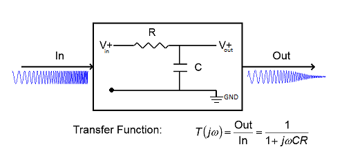
RC low-pass filter circuit with series resistor and shunt capacitor, input chirp, attenuated output, and transfer function T(jw) = 1/(1+jwCR)

You can use the stimulus and the measured waveforms to estimate the transfer function of the R-C circuit, and compare the measured response with the theoretical response of the R-C circuit.

Discover Devices Connected to Your System

daqlist("adi")

ans = 1×4 table
    "SMU1"    "Analog Devices Inc. ADALM1000"    "ADALM1000"    1×1 DeviceInfo

Create a DataAcquisition for the ADALM1000 Device

ADIDaq = daq("adi")

ADIDaq = 
DataAcquisition using Analog Devices Inc. hardware:

                     Running: 0
                        Rate: 100000
           NumScansAvailable: 0
            NumScansAcquired: 0
              NumScansQueued: 0
    NumScansOutputByHardware: 0
                   RateLimit: []

Show channels
Show properties and methods

Add Voltage Source and Measurement Channels

The ADALM1000 device is can source and measure voltage simultaneously on separate channels. Set up the device in this mode.

To source voltage, add an analog output channel with device ID SMU1 and channel ID A, and set its measurement type to Voltage.

addoutput(ADIDaq,'smu1','a','Voltage');

To measure voltage, add an analog input channel with device ID SMU1 and channel ID B, and set its measurement type to Voltage.

addinput(ADIDaq,'smu1','b','Voltage');

Confirm the configuration of the channels.

ADIDaq.Channels

ans = 1×2 object
    1×1 AnalogOutputVoltageChannel    1×1 AnalogInputVoltageChannel

Define and Visualize a Chirp Waveform for Stimulating the Circuit

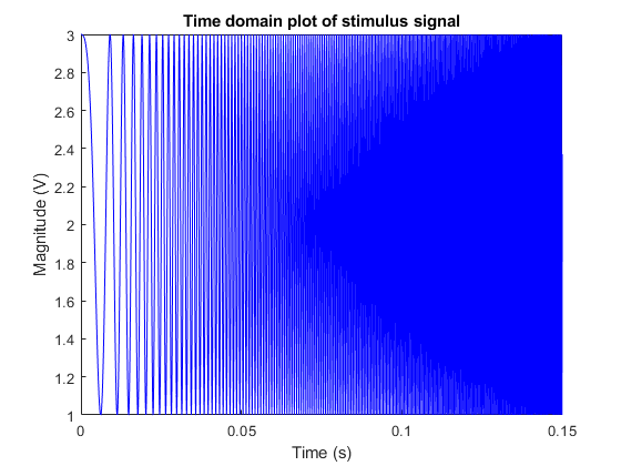
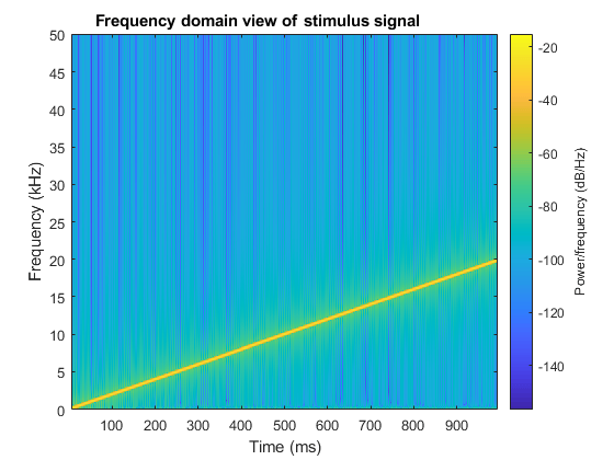
Use a chirp waveform of 1 volt amplitude, ranging in frequency from 20 Hz to 20 kHz for stimulating the circuit. The chirp occurs in a period of 1 second.

Fs = ADIDaq.Rate;
T = 0:1/Fs:1;
ExcitationSignal = chirp(T,20,1,20e3,'linear');

Add a DC offset of 2 V to ensure that the output voltage of the device is always above 0 V.

Offset = 2;
ExcitationSignal = ExcitationSignal + Offset;

Visualize the stimulus signal in the time-domain.

figure(1)
plot(T, ExcitationSignal,'Blue')
xlim([0 0.15])
xlabel('Time (s)')
ylabel('Magnitude (V)')
title('Time domain plot of stimulus signal')

Chirp stimulus signal from 1 to 3 V with increasing frequency over 0 to 0.15 s

Visualize the stimulus signal in the frequency domain.

figure(2)
spectrogram(ExcitationSignal,1024,1000,1024,Fs,'yaxis')
title('Frequency domain view of stimulus signal')

Stimulate the Circuit and Simultaneously Measure the Frequency Response

Generate device output and measure the voltage across the capacitor at the same time on the other channel.

MeasuredTable = readwrite(ADIDaq,ExcitationSignal');
MeasuredSignal = MeasuredTable{:,1};

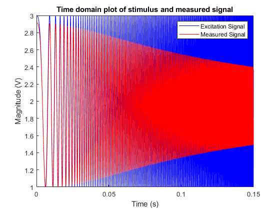
Plot the Stimulus and the Measured Signals

figure(1)
hold on;
plot(T,MeasuredSignal,'Red');
xlim([0 0.15])
ylim([1 3])
title('Time domain plot of stimulus and measured signal')
legend('Excitation Signal','Measured Signal')

Blue excitation signal and red measured signal overlaid, showing increasing attenuation of the measured signal at higher frequencies

figure(3)
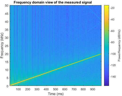
spectrogram(MeasuredSignal,1024,1000,1024,Fs,'yaxis')
title('Frequency domain view of the measured signal')

Spectrogram of the measured signal showing power concentrated along a diagonal line from 0 to 20 kHz over 1 second

Calculate the Transfer Function of the Circuit

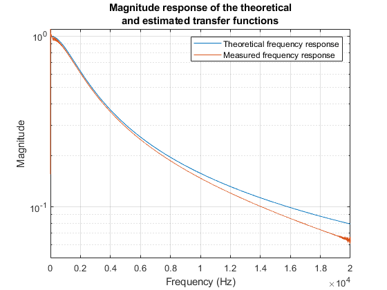
To calculate the transfer function of the R-C circuit, compare the measured signal and the stimulus signal, and plot the magnitude response.

Remove DC offset before processing.

MeasuredSignal = MeasuredSignal - mean(MeasuredSignal);
ExcitationSignal = ExcitationSignal - Offset;
[TFxy,Freq] = tfestimate(ExcitationSignal,MeasuredSignal,[],[],[],Fs);
Mag = abs(TFxy);

Compare the estimated transfer function with the theoretical magnitude response.

R = 1000;    % Resistance (ohms)
C = 0.1e-6;  % Capacitance (farads)
TFMagTheory = abs(1./(1 + (1i*2*pi*Freq*C*R)));

figure(4);
semilogy(Freq,TFMagTheory,Freq,Mag);
xlim([0 20e3])
xlabel('Frequency (Hz)')
ylim([0.05 1.1])
ylabel('Magnitude')
grid on
legend('Theoretical frequency response','Measured frequency response')
title({'Magnitude response of the theoretical'; 'and estimated transfer functions'});

Semilog magnitude plot comparing theoretical and measured frequency responses of the RC circuit, both rolling off from 0 to 20 kHz

Clear the DataAcquisition and Figures

clear ADIDaq
close all