Train Network Using Automatic Multi-GPU Support
This example shows how to use multiple GPUs on your local machine for deep learning training using automatic parallel support.
Training deep learning networks often takes hours or days. With parallel computing, you can speed up training using multiple GPUs. To learn more about options for parallel training, see Scale Up Deep Learning in Parallel, on GPUs, and in the Cloud.
Requirements
Before you can run this example, you must download the CIFAR-10 data set to your local machine. To download the CIFAR-10 data set, use the downloadCIFARToFolders function, attached to this example as a supporting file. To access this file, open the example as a live script. The following code downloads the data set to your current directory. If you already have a local copy of CIFAR-10, then you can skip this section.
directory = pwd;
[locationCifar10Train,locationCifar10Test] = downloadCIFARToFolders(directory);
Downloading CIFAR-10 data set...done.
Copying CIFAR-10 to folders...done.
Load Data Set
Load the training and test data sets by using an imageDatastore object and extract the names of the classes. In the following code, ensure that the location of the datastores points to CIFAR-10 in your local machine.
imdsTrain = imageDatastore(locationCifar10Train, ...
 IncludeSubfolders=true, ...
 LabelSource="foldernames");

imdsTest = imageDatastore(locationCifar10Test, ...
 IncludeSubfolders=true, ...
 LabelSource="foldernames");

classNames = categories(imdsTrain.Labels);
To train the network with augmented image data, create an augmentedImageDatastore object. Use random translations and horizontal reflections. Data augmentation helps prevent the network from overfitting and memorizing the exact details of the training images.
imageSize = [32 32 3];
pixelRange = [-4 4];
imageAugmenter = imageDataAugmenter( ...
    RandXReflection=true, ...
    RandXTranslation=pixelRange, ...
    RandYTranslation=pixelRange);
augmentedImdsTrain = augmentedImageDatastore(imageSize,imdsTrain, ...
    DataAugmentation=imageAugmenter);
Define Network Architecture and Training Options
Define a network architecture for the CIFAR-10 data set. To simplify the code, use convolutional blocks that convolve the input. The pooling layers downsample the spatial dimensions.
blockDepth = 4; % blockDepth controls the depth of a convolutional block.
netWidth = 32; % netWidth controls the number of filters in a convolutional block.

layers = [
    imageInputLayer(imageSize)

    convolutionalBlock(netWidth,blockDepth)
    maxPooling2dLayer(2,Stride=2)
    convolutionalBlock(2*netWidth,blockDepth)
    maxPooling2dLayer(2,Stride=2)
    convolutionalBlock(4*netWidth,blockDepth)
    averagePooling2dLayer(8)

    fullyConnectedLayer(10)
    softmaxLayer];
Specify the training options.
Train the network using multiple GPUs by setting the execution environment to "
multi-gpu". When you use multiple GPUs, you increase the available computational resources. Scale up the mini-batch size with the number of GPUs to keep the workload on each GPU constant. In this example, the number of GPUs is two. Scale the learning rate according to the mini-batch size. Training on a GPU requires a Parallel Computing Toolbox™ license and a supported GPU device. For information on supported devices, see GPU Computing Requirements (Parallel Computing Toolbox).Use a learning rate schedule to drop the learning rate as the training progresses.
Turn on the training progress plot to obtain visual feedback during training.
numGPUs = gpuDeviceCount("available")numGPUs = 4
miniBatchSize = 256*numGPUs;
initialLearnRate = 1e-1*miniBatchSize/256;

options = trainingOptions("sgdm", ...
    ExecutionEnvironment="multi-gpu", ... % Turn on automatic multi-gpu support.
    InitialLearnRate=initialLearnRate, ... % Set the initial learning rate.
    MiniBatchSize=miniBatchSize, ... % Set the MiniBatchSize.
    Verbose=false, ... % Do not send command line output.
    Plots="training-progress", ... % Turn on the training progress plot.
    Metrics="accuracy", ...
    L2Regularization=1e-10, ...
    MaxEpochs=60, ...
    Shuffle="every-epoch", ...
    ValidationData=imdsTest, ...
    ValidationFrequency=floor(4*numel(imdsTrain.Files)/miniBatchSize), ...
    LearnRateSchedule="piecewise", ...
    LearnRateDropFactor=0.1, ...
    LearnRateDropPeriod=50);
Train Network
Train the neural network using the trainnet function. For classification, use cross-entropy loss.
net = trainnet(augmentedImdsTrain,layers,"crossentropy",options);Starting parallel pool (parpool) using the 'Processes' profile ... Connected to parallel pool with 4 workers.

Automatic multi-GPU support can speed up network training by taking advantage of several GPUs. The following plot shows the speedup in the overall training time with the number of GPUs on a Linux machine with four NVIDIA© TITAN Xp GPUs.

Test Network
Classify the test images. To make predictions using multiple GPUs, divide up the data, and make the predictions in parallel.
Determine the total number of observations in the test data set.
numObservations = numel(imdsTest.Files);
In this example, you can use the parallel pool that opened during training. If you do not have a parallel pool open, open one with as many workers as you have GPUs.
parpool("Processes",numGPUs);
Use parfor (Parallel Computing Toolbox) to classify the images in parallel. A parfor-loop is similar to a for-loop, but the loop iterations are executed in parallel on workers in a parallel pool. Inside the parfor-loop:
Select a subset of the test data using the
subsetfunction.Make predictions using the
minibatchpredictfunction on the subset. Theminibatchpredictfunction automatically uses a GPU if one is available. Otherwise, the function uses the CPU.Convert the prediction scores to labels using the
scores2labelfunction.
parfor idx = 1:numGPUs
	startIdx = ceil((idx-1)*numObservations/numGPUs) + 1;
    endIdx = ceil(idx*numObservations/numGPUs);
    subdsTest = subset(imdsTest,startIdx:endIdx);

    scoresTest = minibatchpredict(net,subdsTest,MiniBatchSize=miniBatchSize);
    YTest{idx} = scores2label(scoresTest,classNames);
end
Collect the predictions into a single array.
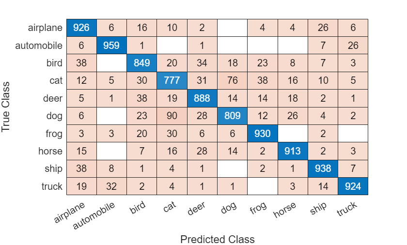
YTest = cat(1,YTest{:});Determine the accuracy of the network and plot a confusion chart.
accuracy = sum(YTest==imdsTest.Labels)/numel(imdsTest.Labels)
accuracy =
0.8853
confusionchart(imdsTest.Labels,YTest)
Define Helper Function
Define a function to create a convolutional block in the network architecture.
function layers = convolutionalBlock(numFilters,numConvLayers)
    layers = [
        convolution2dLayer(3,numFilters,Padding="same")
        batchNormalizationLayer
        reluLayer];

    layers = repmat(layers,numConvLayers,1);
end
See Also
trainnet | trainingOptions | dlnetwork | imageDatastore