View and Compare Code Execution Times

You can run a software-in-the-loop (SIL), processor-in-the-loop (PIL), or XCP-based external mode simulation that produces execution-time metrics for your generated code.

During the simulation, you can use the Simulation Data Inspector to observe streamed execution times. In an XCP-based external mode simulation, you can also visualize task scheduling and related target hardware activity.

At the end of the simulation, you can:

• Use the Code Profile Analyzer to analyze execution-time metrics for profiled model components. You can view, for example, the profiled code section and the execution-time distribution for each profiled code section.

• Open a report of execution-time metrics for profiled components.

• Use the Simulation Data Inspector to plot and compare execution times from various simulations.

Run Simulation That Generates Execution-Time Metrics

In this section, to generate execution-time metrics, you run a SIL simulation. For an example that runs an XCP-based external mode simulation, see Visualize Task Scheduling in XCP External Mode Simulation.

Open the SILTopModel model, which has two subsystems CounterTypeA and CounterTypeB. At the command line, enter:

openExample('ecoder/SILPILVerificationExample', ...
             supportingFile='SILTopModel.slx')

To run a SIL simulation that generates execution-time metrics, on the SIL/PIL tab:

1. In the Mode section, select SIL/PIL Simulation Only.

2. In the Prepare section, specify these settings:

   1. System Under Test — Top model

   2. SIL/PIL Mode — Software-in-the-Loop (SIL)

3. To measure code execution times for the subsystems, in the Prepare section:

   1. Click Settings.

   2. Under Time Profiling:

      • Click the Task Profiling button on. This action selects the Measure task execution time configuration parameter, which provides execution-time metrics for the task generated from the top model SILTopModel.

      • Click the Save Options button until it displays ALL DATA. This action sets the Save options configuration parameter to All data.

      • Click the Functions button until it displays COARSE. This action sets the Measure function execution times configuration parameter to Coarse (referenced models and subsystems only), which provides execution-time metrics for the functions generated from the subsystems CounterTypeA and CounterTypeB.

   3. Under Coverage, click the Coverage Collection button off, which disables code coverage analysis. You collect code coverage data separately from profiling data.

   4. Click the Settings button to open the Configuration Parameters dialog box. On the Data Import/Export pane, clear Single simulation output and then click OK.

4. To view streamed execution times during the simulation, open the Simulation Data Inspector. In the Results section, click .

5. In the Run section, click Run SIL/PIL.

In the MATLAB^® base workspace, the simulation generates a variable with the default name, executionProfile, which stores the execution profiling data. You can specify an alternative name through the Workspace variable configuration parameter.

Note

If the Data Import/Export > Single simulation output check box is selected, the simulation creates the variable in your specified Simulink.SimulationOutput object.

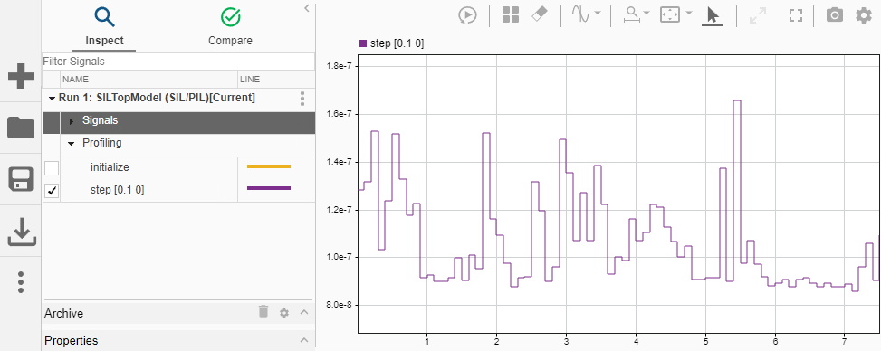
During the simulation, use the Simulation Data Inspector to observe, for example, the variation of execution times for the step function.

When the simulation is complete, the profiled model components are colored blue. For top-model SIL or PIL simulations, the Simulink^® Editor background is also colored blue. The SIL/PIL tab displays two additional panels:

• Profiling details — Provides links to the code execution profiling report or the Code Profile Analyzer.

• Code — Displays the generated code. For example, SILTopModel.c.

To view execution-time metrics for top-model tasks, click the blue-shaded background. Or, for a profiled component, click a blue-shaded block. For example, subsystem CounterTypeB.

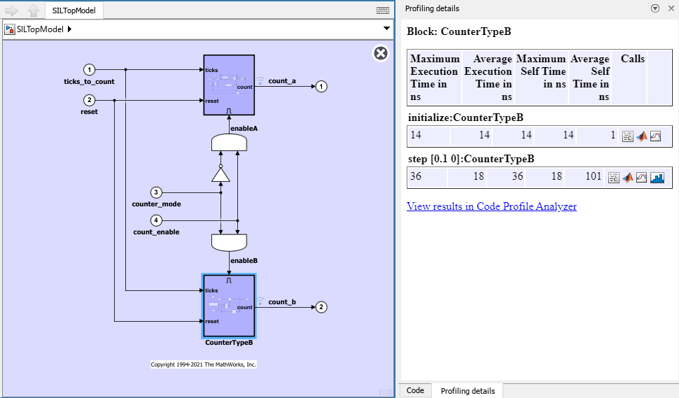
In addition to execution-time metrics, the Profiling details panel provides links to:

• The Code Profile Analyzer, which enables you to view and analyze execution-time metrics for all profiled code sections.

• The Simulation Data Inspector, which allows you to plot and compare execution-time measurements for the profiled code section.

• The execution-time distribution for the profiled code section.

• Pie charts that show the relative execution times of caller and called functions

You can trace from a model component to the profiled code section in the Code view. In the Profiling details panel, on a code section row, click the icon . For example, if you click the model background and then click the icon for the SILTopModel_initialize task, you see the measurement probes around the call site in the SIL application. To see the profiling metrics for the component, place your cursor on the call site.

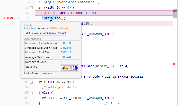
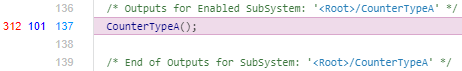
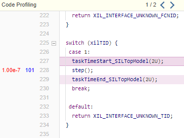
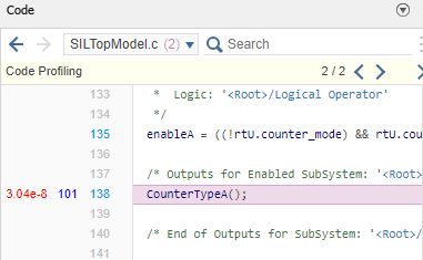
If you click the icon for a function, the call site is highlighted. The Code view displays the average execution time and number of function calls to the left of the code line. In this example, the maximum and average times are the same because the initialization function was called only one time.

If you close the model or display window, you can reopen the colored model and display window with this line command:

annotate(executionProfile)

Analyze Task and Function Execution Times

To open the Code Profile Analyzer:

• Click the SIL/PIL tab.

• In the Results gallery, under Execution Profiling Results, click Code Profile Analyzer.

Or, in the Command Window, enter:

coder.profile.show(executionProfile)

The app displays information in the Task Execution and Summary panels.

View Task Metrics

In the Task Execution panel, the Task Execution Times view shows execution-time metrics for these generated code sections:

• The model initialization function initialize.

• The task represented by the step function step [0.1 0].

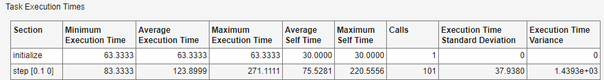
For each code section, the table provides this information:

• Section — Name of profiled code section.

• Minimum Execution Time — Shortest time between start and end of code section.

• Average Execution Time — Average time between start and end of code section.

• Maximum Execution Time — Longest time between start and end of code section.

• Average Self Time — Average execution time, excluding time in child sections.

• Maximum Self Time — Maximum execution time, excluding time in child sections.

• Calls — Number of calls to the code section.

• Execution Time Standard Deviation — A measure of the spread of task execution-times about the average value.

• Execution Time Variance — A measure of the dispersion of execution-time measurements. The execution-time standard deviation is the square root of this value.

By default, the app displays time in nanoseconds (10^-9 seconds). To change the time unit, in the Settings section, from the Time unit drop-down list, select another unit, for example, Microseconds (us).

The table displays time in seconds only if the timer is calibrated, that is, the number of timer ticks per second is known:

• On a Windows^® computer, the software determines this value for a SIL simulation.

• On a Linux^® computer, calibrate the timer manually. In the Settings section, in the CPU Clock (Hz) field, specify your processor speed in Hz.

The Results section of the toolstrip provides features that you can use in your analysis of tasks. For example, to view the step [0.1 0] call in generated code:

1. Click the row that contains step [0.1 0].

2. In the Results section, click Highlight Code. The Simulink Editor displays the call in the Code view.

   

View CPU Workload

The CPU Utilization view provides information about the CPU workload, which enables you to determine whether you can run the generated code on your target hardware.

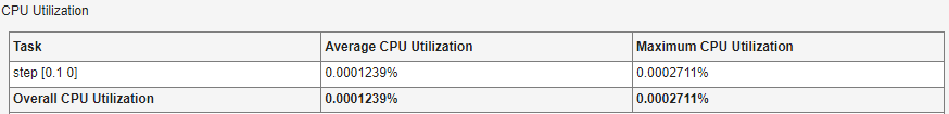
The table provides this information:

• Task — Task name

• Average CPU Utilization — Average CPU time required by each task during a sample period

• Maximum CPU Utilization — Maximum CPU time required by each task during a sample period

• Overall CPU Utilization — Total CPU usage in a sample period.

The software computes the percentage of CPU time assigned to a task by dividing the task execution time by sample time.

The software generates CPU Utilization metrics only if the number of timer ticks per second is known, that is, a value is specified in the CPU Clock (Hz) field.

Summary Panel (Execution-Time)

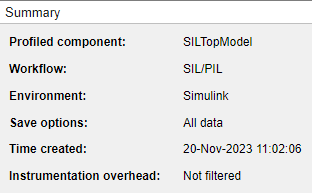
The Summary panel provides miscellaneous simulation information:

• Profiled component — Simulink model that is the source of the generated code

• Workflow — Type of code execution

• Environment — Simulation environment

• Save options — Value of Save options configuration parameter

• Time created — Date and time when workspace variable with execution-time metrics was created

View Function Metrics

On the toolstrip, in the Analysis section, click Function Execution.

The Function Execution Times view provides a function-call tree and execution-time metrics for the tasks and their child functions, that is, the functions generated from subsystems CounterTypeA and CounterTypeB.

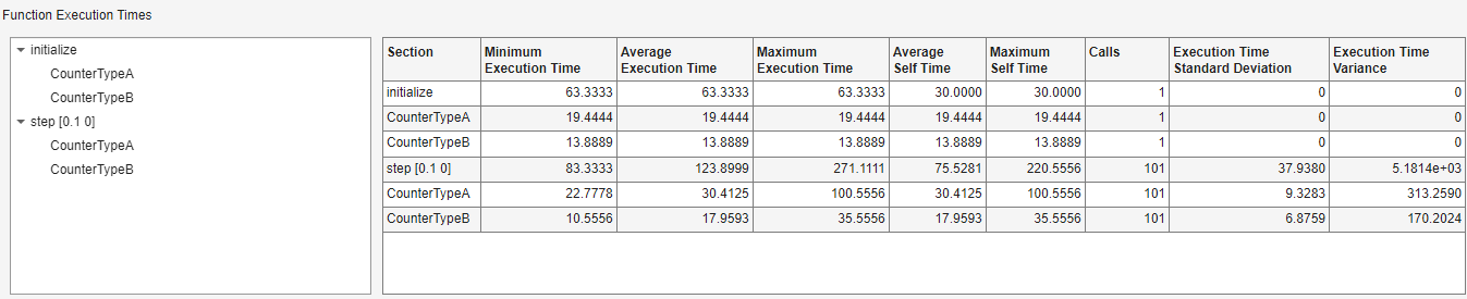
The Relative Function Execution Times view provides function execution times as percentages of caller function and total execution times, which can help you to identify performance bottlenecks in generated code.

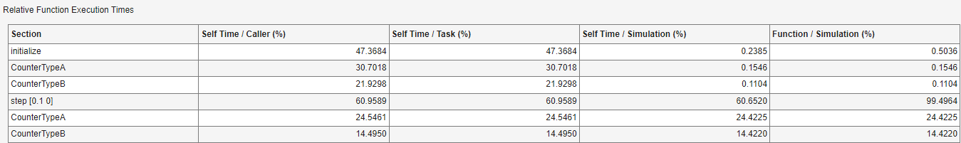
The table contains these metrics.

Column	Comparison Performed
Self Time / Caller (%)	Function self time compared with the total execution time of the caller function.
Self Time / Task (%)	Function self time compared with the total execution time of the task.
Self Time / Simulation (%)	Function self time compared with the total execution time of the simulation.
Function / Simulation (%)	Function execution time, which includes self time and time spent in child functions, compared with the total execution time of the simulation.

The Results section of the toolstrip provides features that you can use in your analysis of functions.

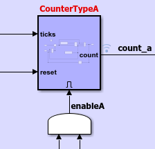
To trace the model component associated with a generated function and its metrics:

1. In the function-call tree or a metrics table, click the function. For example, CounterTypeA, which is called by step [0.1 0].

2. On the toolstrip, in the Results section, click Highlight Source. The Simulink Editor identifies the subsystem.

To view the function call in generated code, in the Results section, click Highlight Code. The Simulink Editor displays the call in the Code view.

To display the execution-time distribution for the function, in the Results section, click Generate Distribution.

CounterTypeA is nested in caller function step [0.1 0]. To view the relative execution times of caller and called functions:

1. In the function-call tree or a metrics table, click the caller function step [0.1 0].

2. On the toolstrip, in the Results section, click Function Distribution, which generates these pie charts.

Use the pie charts to identify functions that are bottlenecks in code execution.

To display measured execution times in the Simulation Data Inspector, in the Results section, click Export to SDI . The Simulation Data Inspector displays execution times for CounterTypeA. Under Filter Signals, if you also select the step [0.1 0] and CounterTypeB check boxes, you can see how execution times for the step and child functions vary over simulation time.

The execution time for the step function step [0 0.1] is the sum of its self-time and execution times for the child functions CounterTypeA and CounterTypeB. You can use the Simulation Data Inspector to manage and compare plots from various simulations.

To view execution-time metrics for the generated code in an HTML report, in the Results section, click Open Report. For more information, see Code Execution Profiling Report.

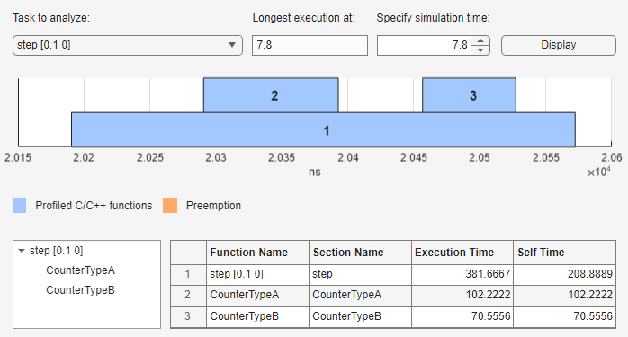
Visualize Function-Call Stack

You can visualize the function call-stack at the simulation step where a task takes longest to execute.

1. On the toolstrip, in the Analysis section, click Function-Call Stack.

2. From the Task to analyze drop-down list, select a code section.

3. Note the Longest execution at field value, the simulation time at which execution of the code section is the longest.

4. Use the default value for Specify simulation time. Modify the value only if you want to visualize the function-call stack at a different simulation time.

5. Click Display.

The panel displays:

• The function-call stack.

• The function-call tree.

• Execution-time and self-time values for profiled code sections.

Compare Execution Times Against Baseline

You can compare execution-time metrics from the current simulation against values from a baseline simulation.

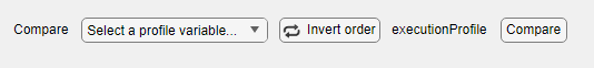
1. On the toolstrip, in the Analysis section, click Comparison.

2. From the Compare current data drop-down list, select the workspace variable that contains results from the baseline simulation. You can update the drop-down list by clicking Refresh list.

3. Click Compare.

The panel displays:

• The function-call tree

• A percentage comparison of execution-time metrics for the two simulations.

The table cells are colored:

• Green if the current execution-time metric is less than the baseline value.

• Yellow if the current execution-time metric is greater than the baseline value.

If the workspace variable for the baseline simulation does not contain data for a code section, the panel displays NaN.

View Code Execution Profiles for Multiple Model Blocks

If you run a top-model simulation that executes multiple Model blocks in SIL or PIL mode with code execution profiling enabled, you can use the Code Profile Analyzer to view execution-time metrics for code generated from the blocks.

1. Open the top model that contains Model blocks. For example, at the command line, enter:

   openExample('ecoder/SILPILVerificationExample', ...
                supportingFile='SILModelBlock.slx')

2. On the SIL/PIL tab, in the Mode section, specify SIL/PIL Simulation Only.

3. In the Prepare section, specify these settings:

   • System Under Test –– Model blocks in SIL/PIL mode

   • Top Model Mode –– Normal

4. Model block Counter A is already configured to run in SIL mode. For Model block Counter B, specify these parameters:

   • Simulation mode –– Software-in-the-loop (SIL)

   • Code interface –– Normal

5. Both Model blocks reference the model SILCounter. To generate execution times for the Model blocks:

   1. Select CounterA or CounterB.

   2. On the Model Block tab, in the Actions section, click Open as Top Model.

   3. On the SIL/PIL tab, in the Settings gallery, click Functions to COARSE, which sets the Measure function execution times configuration parameter for SILCounter to Coarse (referenced models and subsystems only).

6. To run a top-model simulation:

   1. Select the SILModelBlock window.

   2. On the SIL/PIL tab, in the Run section, click Run SIL/PIL.

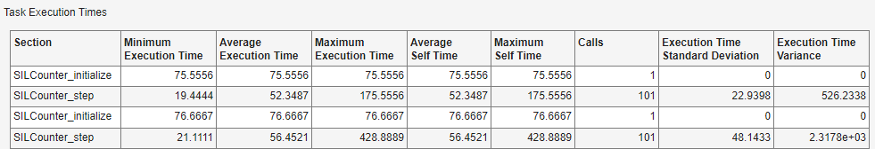
   Since the Single simulation output check box is selected, the simulation creates the variable executionProfile in out, a Simulink.SimulationOutput object.

7. When the simulation is complete, in the Results gallery, under Execution Profiling Results, click Code Profile Analyzer. In the Task Execution panel, the Task Execution Times view shows execution-time metrics for the generated code sections.

   

For information about generating:

• Function execution times for model reference hierarchies, see Control Profiling Granularity.

• Code execution profiling reports for referenced models, see Profiling Reports for Multiple Model Blocks

Visualize Task Scheduling

You can use the Simulation Data Inspector to visualize task scheduling and related target hardware activity.

Simulation Mode	What You Can Observe	How
SIL or PIL	Task scheduling and the order of function calls	When the SIL or PIL simulation is complete, perform one of these actions: In the Results gallery of the Code Profile Analyzer, click Generate Schedule. See Visualize Task Scheduling in SIL Simulation. Run the schedule function. See Visualize Task Scheduling in SIL Simulation. From the SIL/PIL tab, in the Results gallery, click Generate Schedule. See Analyze Results and Export Test Cases.
XCP-based external	Task activity, task diagnostics (run-time only), CPU activity, and CPU utilization	During the XCP external mode simulation, use the Simulation Data Inspector to view displays for task scheduling and related activity. After the simulation, use the schedule function to regenerate displays (except for task diagnostics). For more information, see Visualize Task Scheduling in XCP External Mode Simulation.