Implicitly Create Time-Varying Diffuse State-Space Model
This example shows how to create a diffuse state-space model in which one of the state variables drops out of the model after a certain period.
Suppose that a latent process comprises an AR(2) and an MA(1) model. There are 50 periods, and the MA(1) process drops out of the model for the final 25 periods. Consequently, the state equation for the first 25 periods is
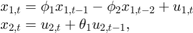
and for the last 25 periods, it is

where  and
and  are Gaussian with mean 0 and standard deviation 1.
The latent processes are measured using
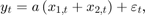
for the first 25 periods, and

for the last 25 periods, where  is Gaussian with mean 0 and standard deviation 1.
Together, the latent process and observation equations make up a state-space model. If the coefficients are unknown parameters, the state-space model is
![$$\begin{array}{l} \left[ {\begin{array}{*{20}{c}} {{x_{1,t}}}\\ {{x_{2,t}}}\\ {{x_{3,t}}}\\ {{x_{4,t}}} \end{array}} \right] = \left[ {\begin{array}{*{20}{c}} {{\phi _1}}&{{\phi _2}}&0&0\\ 1&0&0&0\\ 0&0&0&{{\theta _1}}\\ 0&0&0&0 \end{array}} \right]\left[ {\begin{array}{*{20}{c}} {{x_{1,t - 1}}}\\ {{x_{2,t - 1}}}\\ {{x_{3,t - 1}}}\\ {{x_{4,t - 1}}} \end{array}} \right] + \left[ {\begin{array}{*{20}{c}} 1&0\\ 0&0\\ 0&1\\ 0&1 \end{array}} \right]\left[ {\begin{array}{*{20}{c}} {{u_{1,t}}}\\ {{u_{2,t}}} \end{array}} \right]\\ {y_t} = a({x_{1,t}} + {x_{3,t}}) + {\varepsilon _t} \end{array}$$](../examples/econ/win64/CreateTimeVaryingDiffuseStateSpaceModelExample_eq08939596656225341196.png)
for the first 25 periods,
![$$\begin{array}{l} \left[ {\begin{array}{*{20}{c}} {{x_{1,t}}}\\ {{x_{2,t}}} \end{array}} \right] = \left[ {\begin{array}{*{20}{c}} {{\phi _1}}&{{\phi _2}}&0&0\\ 1&0&0&0 \end{array}} \right]\left[ {\begin{array}{*{20}{c}} {{x_{1,t - 1}}}\\ {{x_{2,t - 1}}}\\ {{x_{3,t - 1}}}\\ {{x_{4,t - 1}}} \end{array}} \right] + \left[ {\begin{array}{*{20}{c}} 1\\ 0 \end{array}} \right]{u_{1,t}}\\ {y_t} = b{x_{1,t}} + {\varepsilon _t} \end{array}$$](../examples/econ/win64/CreateTimeVaryingDiffuseStateSpaceModelExample_eq14434019549381870163.png)
for period 26, and
![$$\begin{array}{l} \left[ {\begin{array}{*{20}{c}} {{x_{1,t}}}\\ {{x_{2,t}}} \end{array}} \right] = \left[ {\begin{array}{*{20}{c}} {{\phi _1}}&{{\phi _2}}\\ 1&0 \end{array}} \right]\left[ {\begin{array}{*{20}{c}} {{x_{1,t - 1}}}\\ {{x_{2,t - 1}}} \end{array}} \right] + \left[ {\begin{array}{*{20}{c}} 1\\ 0 \end{array}} \right]{u_{1,t}}\\ {y_t} = b{x_{1,t}} + {\varepsilon _t} \end{array}$$](../examples/econ/win64/CreateTimeVaryingDiffuseStateSpaceModelExample_eq14967989555778478098.png)
for the last 24 periods.
Write a function that specifies how the parameters in params map to the state-space model matrices, the initial state values, and the type of state.
% Copyright 2015 The MathWorks, Inc.

function [A,B,C,D,Mean0,Cov0,StateType] = diffuseAR2MAParamMap(params,T)
%diffuseAR2MAParamMap Time-variant diffuse state-space model parameter
%mapping function
%
% This function maps the vector params to the state-space matrices (A, B,
% C, and D) and the type of state (StateType). From periods 1 to T/2, the
% state model is an AR(2) and an MA(1) model, and the observation model is
% the sum of the two states. From periods T/2 + 1 to T, the state model is
% just the AR(2) model.  The AR(2) model is diffuse.
    A1 = {[params(1) params(2) 0 0; 1 0 0 0; 0 0 0 params(3); 0 0 0 0]};
    B1 = {[1 0; 0 0; 0 1; 0 1]};
    C1 = {params(4)*[1 0 1 0]};
    Mean0 = [];
    Cov0 = [];
    StateType = [2 2 0 0];
    A2 = {[params(1) params(2) 0 0; 1 0 0 0]};
    B2 = {[1; 0]};
    A3 = {[params(1) params(2); 1 0]};
    B3 = {[1; 0]};
    C3 = {params(5)*[1 0]};
    A = [repmat(A1,T/2,1);A2;repmat(A3,(T-2)/2,1)];
    B = [repmat(B1,T/2,1);B2;repmat(B3,(T-2)/2,1)];
    C = [repmat(C1,T/2,1);repmat(C3,T/2,1)];
    D = 1;
end
Save this code as a file named diffuseAR2MAParamMap on your MATLAB® path.
Create the diffuse state-space model by passing the function diffuseAR2MAParamMap as a function handle to dssm. This example uses 50 observations.
T = 50;
Mdl = dssm(@(params)diffuseAR2MAParamMap(params,T));
dssm implicitly creates the diffuse state-space model. Usually, you cannot verify diffuse state-space models that are implicitly created.
dssm contains unknown parameters. You can simulate data and then estimate parameters using estimate.