filter
Forward recursion of diffuse state-space models
Description
X = filter(Mdl,Y)X)
by performing forward recursion of the fully specified diffuse state-space
model Mdl. That is, filter applies
the diffuse Kalman filter using Mdl and
the observed responses Y.
X = filter(Mdl,Y,Name,Value)Name,Value pair
arguments. For example, specify the regression coefficients and predictor
data to deflate the observations, or specify to use the univariate
treatment of a multivariate model.
If Mdl is not fully specified, then you must
specify the unknown parameters as known scalars using the 'Params' Name,Value pair
argument.
[ additionally returns the loglikelihood
value (X,logL,Output]
= filter(___)logL) and an output structure array (Output)
using any of the input arguments in the previous syntaxes. Output contains:
Filtered and forecasted states
Estimated covariance matrices of the filtered and forecasted states
Loglikelihood value
Forecasted observations and its estimated covariance matrix
Adjusted Kalman gain
Vector indicating which data the software used to filter
Input Arguments
Name-Value Arguments
Output Arguments
Examples
Suppose that a latent process is a random walk. The state equation is
where is Gaussian with mean 0 and standard deviation 1.
Generate a random series of 100 observations from , assuming that the series starts at 1.5.
T = 100;
x0 = 1.5;
rng(1); % For reproducibility
u = randn(T,1);
x = cumsum([x0;u]);
x = x(2:end);
Suppose further that the latent process is subject to additive measurement error. The observation equation is
where is Gaussian with mean 0 and standard deviation 0.75. Together, the latent process and observation equations compose a state-space model.
Use the random latent state process (x) and the observation equation to generate observations.
y = x + 0.75*randn(T,1);
Specify the four coefficient matrices.
A = 1;
B = 1;
C = 1;
D = 0.75;
Create the diffuse state-space model using the coefficient matrices. Specify that the initial state distribution is diffuse.
Mdl = dssm(A,B,C,D,'StateType',2)Mdl =
State-space model type: dssm
State vector length: 1
Observation vector length: 1
State disturbance vector length: 1
Observation innovation vector length: 1
Sample size supported by model: Unlimited
State variables: x1, x2,...
State disturbances: u1, u2,...
Observation series: y1, y2,...
Observation innovations: e1, e2,...
State equation:
x1(t) = x1(t-1) + u1(t)
Observation equation:
y1(t) = x1(t) + (0.75)e1(t)
Initial state distribution:
Initial state means
x1
0
Initial state covariance matrix
x1
x1 Inf
State types
x1
Diffuse
Mdl is an dssm model. Verify that the model is correctly specified using the display in the Command Window.
Filter states for periods 1 through 100. Plot the true state values and the filtered state estimates.
filteredX = filter(Mdl,y);

figure
plot(1:T,x,'-k',1:T,filteredX,':r','LineWidth',2)
title({'State Values'})
xlabel('Period')
ylabel('State')
legend({'True state values','Filtered state values'})
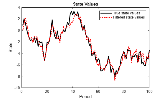
The true values and filter estimates are approximately the same, except for the first filtered state, which is zero.
Suppose that the linear relationship between unemployment rate and the nominal gross national product (nGNP) is of interest. Suppose further that unemployment rate is an AR(1) series. Symbolically, and in state-space form, the model is
where:
is the unemployment rate at time t.
is the observed change in the unemployment rate being deflated by the return of nGNP ().
is the Gaussian series of state disturbances having mean 0 and unknown standard deviation .
Load the Nelson-Plosser data set, which contains the unemployment rate and nGNP series, among other things.
load Data_NelsonPlosserPreprocess the data by taking the natural logarithm of the nGNP series, and removing the starting NaN values from each series.
isNaN = any(ismissing(DataTable),2);       % Flag periods containing NaNs
gnpn = DataTable.GNPN(~isNaN);
y = diff(DataTable.UR(~isNaN));
T = size(gnpn,1);                          % The sample size
Z = price2ret(gnpn);
This example continues using the series without NaN values. However, using the Kalman filter framework, the software can accommodate series containing missing values.
Specify the coefficient matrices.
A = NaN;
B = NaN;
C = 1;
Create the state-space model using dssm by supplying the coefficient matrices and specifying that the state values come from a diffuse distribution. The diffuse specification indicates complete ignorance about the moments of the initial distribution.
StateType = 2;
Mdl = dssm(A,B,C,'StateType',StateType);
Estimate the parameters. Specify the regression component and its initial value for optimization using the 'Predictors' and 'Beta0' name-value pair arguments, respectively. Display the estimates and all optimization diagnostic information. Restrict the estimate of to all positive, real numbers.
params0 = [0.3 0.2]; % Initial values chosen arbitrarily
Beta0 = 0.1;
[EstMdl,estParams] = estimate(Mdl,y,params0,'Predictors',Z,'Beta0',Beta0,...
    'lb',[-Inf 0 -Inf]);
Method: Maximum likelihood (fmincon)
Effective Sample size:             60
Logarithmic  likelihood:     -110.477
Akaike   info criterion:      226.954
Bayesian info criterion:      233.287
           |      Coeff       Std Err    t Stat    Prob
--------------------------------------------------------
 c(1)      |   0.59436       0.09408     6.31738  0
 c(2)      |   1.52554       0.10758    14.17991  0
 y <- z(1) | -24.26161       1.55730   -15.57930  0
           |
           |    Final State   Std Dev     t Stat   Prob
 x(1)      |   2.54764        0           Inf     0
EstMdl is an ssm model, and you can access its properties using dot notation.
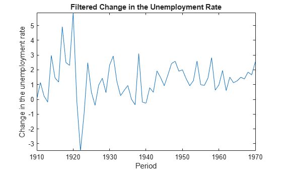
Filter the estimated diffuse state-space model. EstMdl does not store the data or the regression coefficients, so you must pass in them in using the name-value pair arguments 'Predictors' and 'Beta', respectively. Plot the estimated, filtered states.
filteredX = filter(EstMdl,y,'Predictors',Z,'Beta',estParams(end));

figure
plot(dates(end-(T-1)+1:end),filteredX);
xlabel('Period')
ylabel('Change in the unemployment rate')
title('Filtered Change in the Unemployment Rate')
axis tight
Estimate a diffuse state-space model, filter the states, and then extract other estimates from the Output output argument.
Consider the diffuse state-space model
The state variable is an AR(1) model with autoregressive coefficient . is a random walk. The disturbances and are independent Gaussian random variables with mean 0 and standard deviations and , respectively. The observation is the error-free sum of and .
Generate data from the state-space model. To simulate the data, suppose that the sample size , , , , and .
rng(1); % For reproducibility
T = 100;
ARMdl = arima('AR',0.6,'Constant',0,'Variance',0.2^2);
x1 = simulate(ARMdl,T,'Y0',2);
u3 = 0.1*randn(T,1);
x3 = cumsum([2;u3]);
x3 = x3(2:end);
y = x1 + x3;
Specify the coefficient matrices of the state-space model. To indicate unknown parameters, use NaN values.
A = [NaN 0; 0 1];
B = [NaN 0; 0 NaN];
C = [1 1];
Create a diffuse state-space model that describes the model above. Specify that and have diffuse initial state distributions.
StateType = [2 2];
Mdl = dssm(A,B,C,'StateType',StateType);
Estimate the unknown parameters of Mdl. Choose initial parameter values for optimization. Specify that the standard deviations are constrained to be positive, but all other parameters are unconstrained using the 'lb' name-value pair argument.
params0 = [0.01 0.1 0.01]; % Initial values chosen arbitrarily
EstMdl = estimate(Mdl,y,params0,'lb',[-Inf 0 0]);
Method: Maximum likelihood (fmincon)
Effective Sample size:             98
Logarithmic  likelihood:      3.44283
Akaike   info criterion:    -0.885655
Bayesian info criterion:      6.92986
      |     Coeff      Std Err   t Stat     Prob
--------------------------------------------------
 c(1) | 0.54134       0.20494    2.64145  0.00826
 c(2) | 0.18439       0.03305    5.57897   0
 c(3) | 0.11783       0.04347    2.71039  0.00672
      |
      |  Final State   Std Dev    t Stat    Prob
 x(1) | 0.24884       0.17168    1.44943  0.14722
 x(2) | 1.73762       0.17168   10.12121   0
The parameters are close to their true values.
Filter the states of EstMdl, and request all other available output.
[X,logL,Output] = filter(EstMdl,y);
X is a T-by-2 matrix of filtered states, logL is the final optimized log-likelihood value, and Output is a structure array containing various estimates that the Kalman filter requires. List the fields of output using fields.
fields(Output)
ans = 9×1 cell
    {'LogLikelihood'      }
    {'FilteredStates'     }
    {'FilteredStatesCov'  }
    {'ForecastedStates'   }
    {'ForecastedStatesCov'}
    {'ForecastedObs'      }
    {'ForecastedObsCov'   }
    {'KalmanGain'         }
    {'DataUsed'           }
Convert Output to a table.
OutputTbl = struct2table(Output);
OutputTbl(1:10,1:5) % Display first ten rows of first five variablesans=10×5 table
LogLikelihood FilteredStates FilteredStatesCov ForecastedStates ForecastedStatesCov
_____________ ______________ _________________ ________________ ___________________
{0×0 double} {0×0 double} {0×0 double} {0×0 double} {0×0 double}
{0×0 double} {0×0 double} {0×0 double} {0×0 double} {0×0 double}
{[ 0.1827]} {2×1 double} {2×2 double} {2×1 double} {2×2 double}
{[ 0.0972]} {2×1 double} {2×2 double} {2×1 double} {2×2 double}
{[ 0.4472]} {2×1 double} {2×2 double} {2×1 double} {2×2 double}
{[ 0.2073]} {2×1 double} {2×2 double} {2×1 double} {2×2 double}
{[ 0.5167]} {2×1 double} {2×2 double} {2×1 double} {2×2 double}
{[ 0.2389]} {2×1 double} {2×2 double} {2×1 double} {2×2 double}
{[ 0.5064]} {2×1 double} {2×2 double} {2×1 double} {2×2 double}
{[ -0.0105]} {2×1 double} {2×2 double} {2×1 double} {2×2 double}
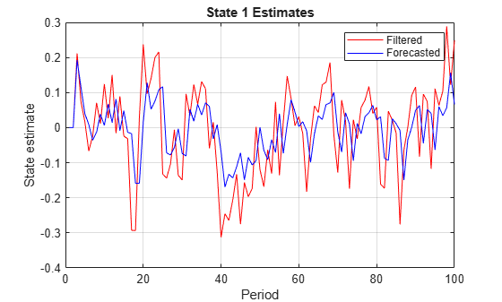
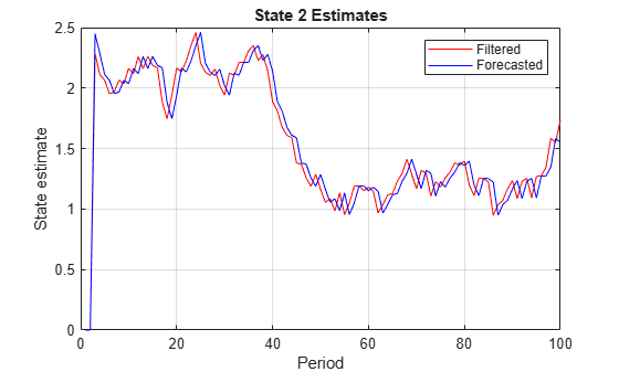
The first two rows of the table contain empty cells or zeros. These correspond to the observations required to initialize the diffuse Kalman filter. That is, SwitchTime is 2.
SwitchTime = 2;
Plot the filtered and forecasted states.
ForeX = cell2mat(OutputTbl.ForecastedStates')'; % Orient forecasted states
ForeX = [zeros(SwitchTime,2);ForeX]; % Include zeros for initialization

figure;
plot(1:T,X(:,1),'r',1:T,ForeX(:,1),'b');
xlabel('Period');
ylabel('State estimate');
title('State 1 Estimates')
legend('Filtered','Forecasted');
grid on;
figure;
plot(1:T,X(:,2),'r',1:T,ForeX(:,2),'b');
xlabel('Period');
ylabel('State estimate');
title('State 2 Estimates')
legend('Filtered','Forecasted');
grid on;
Tips
Mdldoes not store the response data, predictor data, and the regression coefficients. Supply the data wherever necessary using the appropriate input or name-value pair arguments.It is a best practice to allow
filterto determine the value ofSwitchTime. However, in rare cases, you might experience numerical issues during estimation, filtering, or smoothing diffuse state-space models. For such cases, try experimenting with variousSwitchTimespecifications, or consider a different model structure (e.g., simplify or reverify the model). For example, convert the diffuse state-space model to a standard state-space model usingssm.To accelerate estimation for low-dimensional, time-invariant models, set
'Univariate',true. Using this specification, the software sequentially updates rather then updating all at once during the filtering process.
Algorithms
The Kalman filter accommodates missing data by not updating filtered state estimates corresponding to missing observations. In other words, suppose there is a missing observation at period t. Then, the state forecast for period t based on the previous t – 1 observations and filtered state for period t are equivalent.
For explicitly defined state-space models,
filterapplies all predictors to each response series. However, each response series has its own set of regression coefficients.The diffuse Kalman filter requires presample data. If missing observations begin the time series, then the diffuse Kalman filter must gather enough nonmissing observations to initialize the diffuse states.
For diffuse state-space models,
filterusually switches from the diffuse Kalman filter to the standard Kalman filter when the number of cumulative observations and the number of diffuse states are equal. However, if a diffuse state-space model has identifiability issues (e.g., the model is too complex to fit to the data), thenfiltermight require more observations to initialize the diffuse states. In extreme cases,filterrequires the entire sample.
References
[1] Durbin J., and S. J. Koopman. Time Series Analysis by State Space Methods. 2nd ed. Oxford: Oxford University Press, 2012.
Version History
Introduced in R2015b