Bootstrapping a Default Probability Curve

This example shows how to bootstrap default probabilities from CDS market quotes. To bootstrap default probabilities from bond market data, see bondDefaultBootstrap. In a typical workflow, pricing a new CDS contract involves first estimating a default probability term structure using cdsbootstrap. This requires market quotes of existing CDS contracts, or quotes of CDS indices (e.g., iTraxx). The estimated default probability curve is then used as input to cdsspread or cdsprice. If the default probability information is already known, cdsbootstrap can be bypassed and cdsspread or cdsprice can be called directly.

The market information in this example is provided in the form of running spreads of CDS contracts maturing on the CDS standard payment dates closest to 1, 2, 3, 5, and 7 years from the valuation date.

Settle = '17-Jul-2009'; % valuation date for the CDS
MarketDates = datenum({'20-Sep-10','20-Sep-11','20-Sep-12','20-Sep-14',...
'20-Sep-16'});
MarketSpreads = [140 175 210 265 310]';
MarketData = [MarketDates MarketSpreads];
ZeroDates = datenum({'17-Jan-10','17-Jul-10','17-Jul-11','17-Jul-12',...
'17-Jul-13','17-Jul-14'});
ZeroRates = [1.35 1.43 1.9 2.47 2.936 3.311]'/100;
ZeroData = [ZeroDates ZeroRates];

[ProbData,HazData] = cdsbootstrap(ZeroData,MarketData,Settle);

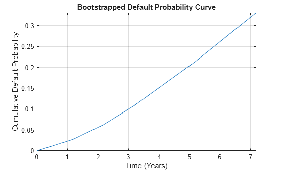
The bootstrapped default probability curve is plotted against time, in years, from the valuation date.

ProbTimes = yearfrac(Settle,ProbData(:,1));
figure
plot([0; ProbTimes],[0; ProbData(:,2)])
grid on
axis([0 ProbTimes(end,1) 0 ProbData(end,2)])
xlabel('Time (years)')
ylabel('Cumulative Default Probability')
title('Bootstrapped Default Probability Curve')

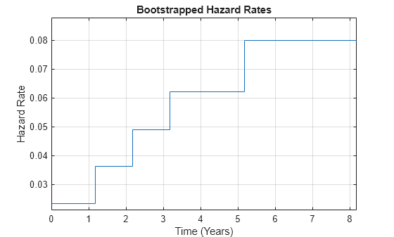
The associated hazard rates are returned as an optional output. The convention is that the first hazard rate applies from the settlement date to the first market date, the second hazard rate from the first to the second market date, and so on, and the last hazard rate applies from the second-to-last market date onwards. The following plot displays the bootstrapped hazard rates, plotted against time, in years, from the valuation date:

HazTimes = yearfrac(Settle,HazData(:,1));
figure
stairs([0; HazTimes(1:end-1,1); HazTimes(end,1)+1],...
[HazData(:,2);HazData(end,2)])
grid on
axis([0 HazTimes(end,1)+1 0.9*HazData(1,2) 1.1*HazData(end,2)])
xlabel('Time (years)')
ylabel('Hazard Rate')
title('Bootstrapped Hazard Rates')