Role of Convexity in Portfolio Problems

When using a Portfolio object and the estimateCustomObjectivePortfolio function with the Financial Toolbox™ solvers, the solvers return a local minimum, which is not guaranteed to be a global minimum. A local minimum of a function is a point where the function value is smaller than the points around it, but the value is larger than a distant point. A global minimum is the point where the function value is smaller than at all other points. Convex functions play an important role in optimization because they guarantee that all local minima are global minima. In other words, any solution found by the solver is guaranteed to be a global minimum.

Another important feature of convex functions is that all tangents of the function lie underneath the function. This feature is particularly useful in problems with cardinality constraints or conditional bounds. For more information on cardinality constraints and conditional bounds, see Working with 'Conditional' BoundType, MinNumAssets, and MaxNumAssets Constraints Using Portfolio Objects and setMinMaxNumAssets. The Financial Toolbox internal solvers for portfolio problems with binary variables use an iterative method that approximates the nonlinear functions (for example, variance) with a collection of linear functions. The linear functions used to approximate the original function are the tangents of the function at different points. Because the tangents for convex functions always lie underneath the function, the Financial Toolbox solvers guarantee that the approximation does not remove any minimum from the problem.

Using Financial Toolbox solvers for portfolio problems with nonconvex functions and cardinality constraints or conditional bounds might result in suboptimal solutions. The reason is that the tangent lines used to approximate the nonconvex functions might cut off different minima as demonstrated in the following figure:

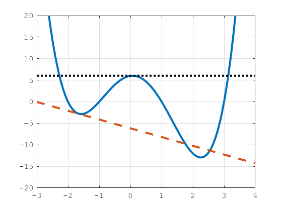
Even though the red dashed tangent line cuts off only a small piece of the graph, that small piece already contains an important point, the global minima. In the worst case scenario, the Financial Toolbox solvers compute the tangent line at a point that removes all minima of the function, like the black dotted line does. Therefore, it is important to be aware of the type of function passed to a Financial Toolbox solver.

All the above applies to minimization problems. Conversely, maximization problems with cardinality constraints or conditional bounds can be solved by the Financial Toolbox solvers only if the functions are concave.

Examples of Convex Functions

Here are some examples of common convex functions used in finance. You can use these convex functions in minimization problems when using a Portfolio object with the estimateCustomObjectivePortfolio function:

• Variance:

  $$x^T\Sigma x$$

• Tracking error:

  $${(x-x_0)}^T\Sigma (x-x_0)$$

• Herfindahl-Hirschman index:

  $$x^{T}x$$

• Any linear function

• Any positive combination of convex functions:

  $$\begin{array}{l}{x}^T\Sigma x+\lambda {(}^x\Sigma (x-x_0),\lambda \ge 0\\ x^T\Sigma x+{\lambda }_1{x}^{T}x+{\lambda }_2{(}^x\Sigma (x-x_0),{\lambda }_1,{\lambda }_2\ge 0\end{array}$$

Note

If the portfolio problem has cardinality constraints or conditional bounds specified using setMinMaxNumAssets or setBounds, the objective function must also be convex.

Examples of Concave Functions

Here are some examples of common concave functions used in finance. You can use concave functions in maximization problems when using a Portfolio object with the estimateCustomObjectivePortfolio function.

• Risk penalized return:

  $${\mu }^{T}x-\lambda x^T\Sigma x,\lambda \ge \text{0}$$

• Any linear function

• Any positive combination of concave functions

Examples of Nonconvex Functions

Here are some examples of common nonconvex functions used in finance. You can use nonconvex functions in minimization or maximization problems when using a Portfolio object without cardinality constraints or conditional bounds with the estimateCustomObjectivePortfolio function.

• Sharpe ratio:

  $$\frac{{\mu }^{T}x-r_f}{\sqrt{x^T\Sigma x}}$$

• Information ratio:

  $$\frac{{\mu }^T(x-x_0)}{\sqrt{{(x-x_0)}^T\Sigma (x-x_0)}}$$

• Diversification ratio:

  $$\frac{{\sigma }^{T}x}{\sqrt{x^T\Sigma x}}$$

• Risk budgeting deviation:

  $${{\displaystyle \sum _i\left(\frac{x_i{(\Sigma x)}_i}{x^T\Sigma x}-b_i\right)}}^2$$

• The following function is a special case:

  $$x^T\Sigma x-\lambda {\displaystyle \sum _i\ln x_i}$$

  This function is commonly used to construct risk parity portfolios. Although this function is convex, problems with cardinality constraints or conditional bounds make this function ill-defined. This happens because lnx_i is not defined when x_i = 0. Since adding cardinality constraints or conditional bounds imply that some assets have a weight of 0, the function becomes ill-defined at the points of interest.

Note

If the portfolio problem has cardinality constraints or conditional bounds specified using setMinMaxNumAssets or setBounds, the objective function cannot be nonconvex.