Portfolio Selection and Risk Aversion

Introduction

One of the factors to consider when selecting the optimal portfolio for a particular investor is the degree of risk aversion. This level of aversion to risk can be characterized by defining the investor's indifference curve. This curve consists of the family of risk/return pairs defining the trade-off between the expected return and the risk. It establishes the increment in return that a particular investor requires to make an increment in risk worthwhile. Typical risk aversion coefficients range from 2.0 through 4.0, with the higher number representing lesser tolerance to risk. The equation used to represent risk aversion in Financial Toolbox™ software is

U = E(r) - 0.005*A*sig^2

where:

U is the utility value.

E(r) is the expected return.

A is the index of investor's aversion.

sig is the standard deviation.

Note

An alternative to using these portfolio optimization functions is to use the Portfolio object (Portfolio) for mean-variance portfolio optimization. This object supports gross or net portfolio returns as the return proxy, the variance of portfolio returns as the risk proxy, and a portfolio set that is any combination of the specified constraints to form a portfolio set. For information on the workflow when using Portfolio objects, see Portfolio Object Workflow.

Optimal Risky Portfolio

This example shows how to compute the optimal risky portfolio on the efficient frontier based on the risk-free rate, the borrowing rate, and the investor's degree of risk aversion.

You do this with the function portalloc. First generate the efficient frontier data using portopt.

ExpReturn = [0.1 0.2 0.15]; 

ExpCovariance  = [ 0.005   -0.010    0.004;
                  -0.010    0.040   -0.002;
                   0.004   -0.002    0.023];

NumPorts = 20; % Consider 20 different points along the efficient frontier.

[PortRisk, PortReturn, PortWts] = portopt(ExpReturn,... 
ExpCovariance, NumPorts);

Calling portopt, while specifying output arguments, returns the corresponding vectors and arrays representing the risk, return, and weights for each of the portfolios along the efficient frontier. Use these as the first three input arguments to the function portalloc.

Find the optimal risky portfolio and the optimal allocation of funds between the risky portfolio and the risk-free asset, using these values for the risk-free rate, borrowing rate, and investor's degree of risk aversion.

RisklessRate  =  0.08

RisklessRate = 
0.0800

BorrowRate    =  0.12

BorrowRate = 
0.1200

RiskAversion  =  3

RiskAversion = 
3

portalloc(PortRisk, PortReturn, PortWts, RisklessRate,... 
BorrowRate, RiskAversion);

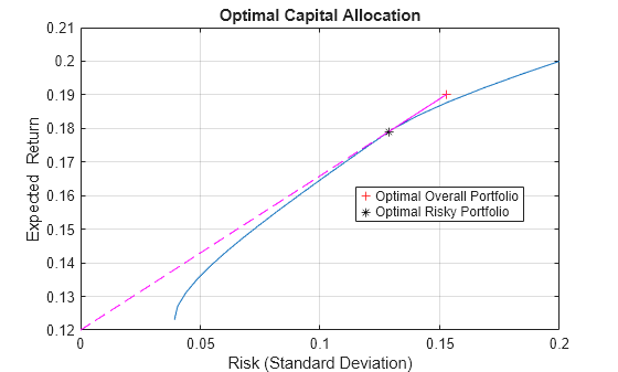
Calling portalloc while specifying the output arguments returns the variance (RiskyRisk), the expected return (RiskyReturn), and the weights (RiskyWts) allocated to the optimal risky portfolio. It also returns the fraction (RiskyFraction) of the complete portfolio allocated to the risky portfolio, and the variance (OverallRisk) and expected return (OverallReturn) of the optimal overall portfolio. The overall portfolio combines investments in the risk-free asset and in the risky portfolio. The actual proportion assigned to each of these two investments is determined by the degree of risk aversion characterizing the investor.

[RiskyRisk, RiskyReturn, RiskyWts,RiskyFraction, OverallRisk, ... 
OverallReturn] = portalloc (PortRisk, PortReturn, PortWts, ... 
RisklessRate, BorrowRate, RiskAversion)

RiskyRisk = 
0.1288

RiskyReturn = 
0.1791

RiskyWts = 1×3

    0.0057    0.5879    0.4064

RiskyFraction = 
1.1869

OverallRisk = 
0.1529

OverallReturn = 
0.1902

The value of RiskyFraction exceeds 1 (100%), implying that the risk tolerance specified allows borrowing money to invest in the risky portfolio, and that no money is invested in the risk-free asset. This borrowed capital is added to the original capital available for investment. In this example, the customer tolerates borrowing 18.69% of the original capital amount.