Explain Black-Box Model Using Fuzzy Support System

This example shows how to develop a fuzzy inference support system that explains the behavior of a black-box model.

Using nondeterministic machine learning methods, such as deep learning, you can design a black-box model to estimate the input-output mapping for a given set of experimental or simulation data. However, the input-output relationship defined by such a black-box model is difficult to understand.

In such cases, a common approach is to create a transparent support system to explain the input-output relationships modeled by the a black box system.

A fuzzy inference system (FIS) is a transparent model that represents system knowledge using an explainable rule base. Since the rule base of a fuzzy system is easier for a user to intuitively understand, a FIS is often used as a support system to explain an existing black box model.

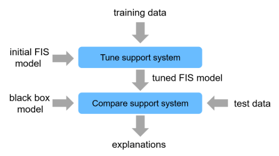
The following figure shows the general steps for developing a fuzzy support system from an existing black box with the assumption that the original training data of the black box is available.

• Tune a support FIS using the original training data for the black box.

• Compare the behavior of the black-box system and the FIS using test data.

• Examine the FIS rules to explain the behavior of the black-box system.

In general, you can uses a fuzzy support system to explain different types of black-box models. For this example, the black-box model is implemented using a deep neural network (DNN), which requires Deep Learning Toolbox™ software.

Black-Box Model

The DNN model for this example imitates an automotive lane keeping assist (LKA) system implemented using model predictive control (MPC). A vehicle (ego car) equipped with an LKA system has a sensor, such as camera, that measures the lateral deviation and relative yaw angle between the centerline of a lane and the ego car. The sensor also measures the current lane curvature and curvature derivative. Depending on the curve length that the sensor can view, the curvature in front of the ego car can be calculated from the current curvature and curvature derivative. The LKA system keeps the ego car travelling along the centerline of the lane by adjusting the front steering angle of the ego car. The goal for lane keeping control is to drive both lateral deviation and relative yaw angle close to zero. For more information on lane keeping using MPC, see Lane Keeping Assist System Using Model Predictive Control (Model Predictive Control Toolbox).

The DNN-based LKA system uses the following inputs to generate the output steering angle ${\mathit{u}}^{*}$.

1. Lateral velocity ${\mathit{V}}_{\mathit{y}}$ m/s

2. Yaw angle rate $\mathit{r}$ rad/s

3. Lateral deviation ${\mathit{e}}_1$ m

4. Relative yaw angle ${\mathit{e}}_2$ rad

5. Previous steering angle (control variable) $\mathit{u}$ rad

6. Measured disturbance (road yaw rate: longitudinal velocity * curvature ($\rho$))

For more information on creating and training the DNN, see Imitate MPC Controller for Lane Keeping Assist (Reinforcement Learning Toolbox).

Download and unzip the data for this example.

dataFile = matlab.internal.examples.downloadSupportFile("fuzzy","FuzzyLKAData.zip");
unzip(dataFile)
data = load('dataExplainDNN.mat');

Obtain the saved DNN model of an LKA system.

dnnLKA = data.trainedDNN;

The trained DNN predicts a steering angle based on the current input values to keep the car along the centerline of a lane. to make a prediction, use the predict function. For example, the following command predicts the steering angle when all input signals are zero.

steeringAngle = predict(dnnLKA,zeros(1,6))

steeringAngle = single
    -0.0195

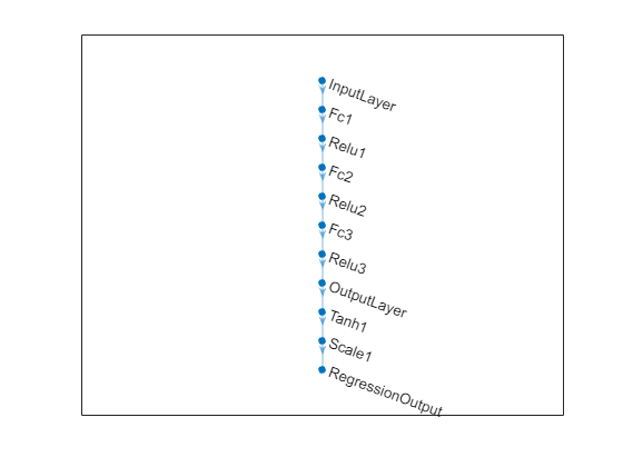
However, the DNN model does not provide any explanation about how it derives the steering angle. The DNN model parameters are the steering angle generation algorithm in terms of hidden units and their associated parameters. Therefore, input-output relations cannot be described using the DNN structure alone.

figure
plot(dnnLKA)

To explain the DNN model behavior, you can create and tune a fuzzy support system.

Create Initial Fuzzy Inference System

For an LKA controller with six inputs, a single monolithic FIS contains a large complex rule base that is difficult to interpret. As an alternative. you can create a FIS tree that incrementally combines input values using multiple FISs, each with a smaller rule base.

Create a FIS tree with four layers and five FISs. Each FIS has two inputs and one output. To create each component FIS, use the constructFIS helper function, which is shown at the end of this example.

numMFs = 2;
fis1 = constructFIS('fis1',numMFs, ...
    data.vRange,data.e1Range,data.uRange,'Vy','e1','u1');
fis2 = constructFIS('fis2',numMFs, ...
    data.rRange,data.e2Range,data.uRange,'r','e2','u2');
fis3 = constructFIS('fis3',numMFs, ...
    data.uRange,data.uRange,data.uRange,'u1','u2','u3');
fis4 = constructFIS('fis4',numMFs, ...
    data.uRange,data.uRange,data.uRange,'u3','u','u4');
fis5 = constructFIS('fis5',numMFs, ...
    data.uRange,data.dRange,data.uRange,'u4','d','u*');

fis = [fis1 fis2 fis3 fis4 fis5];
connections = [...
    fis1.Name+"/"+fis1.Outputs(1).Name fis3.Name+"/"+fis3.Inputs(1).Name; ...
    fis2.Name+"/"+fis2.Outputs(1).Name fis3.Name+"/"+fis3.Inputs(2).Name; ...
    fis3.Name+"/"+fis3.Outputs(1).Name fis4.Name+"/"+fis4.Inputs(1).Name; ...
    fis4.Name+"/"+fis4.Outputs(1).Name fis5.Name+"/"+fis5.Inputs(1).Name ...
    ];

fisTin = fistree(fis,connections);

View the FIS tree structure.

showFISTree(fisTin)

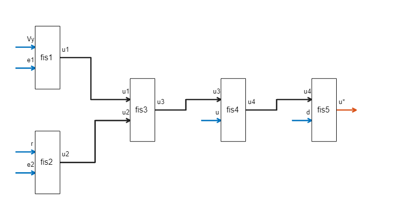
In this FIS tree:

• The first layer uses two FISs: fis1 and fis2, where fis1 combines lateral velocity (${\mathit{V}}_{\mathit{y}}$) and lateral deviation (${\mathit{e}}_1$), and fis2 combines yaw angle ($\mathit{r}$) and relative yaw angle (${\mathit{e}}_2$) to predict expected steering angles ${\mathit{u}}_1$ and ${\mathit{u}}_2$ for the respective input values.

• The second layer uses fis3 to combine the outputs of fis1 and fis2, that is, fis3 combines the effects of lateral displacement and yaw angle to produce a desired steering angle (${\mathit{u}}_3$) for the LKA system.

• The third layer uses fis4 to combine the effect of the previous steering angle ($\mathit{u}$) with the output of second layer to generate ${\mathit{u}}_4$.

• The fourth layer combines the effect of the measured disturbance ($\mathit{d}$) with the desired steering angle predicted by the previous layers using fis5.

Each input of a FIS includes two membership functions (MFs) and each output includes four MFs. As a result, each FIS has four rules and the overall FIS tree has 20 rules.

Tune Fuzzy Inference System

For this example, you tune the FIS in two stages.

1. Establish the input-output relations for each FIS by learning the output membership functions for each possible input combination.

2. Tune the MF parameters for the input and output variables of each FIS.

To learn the output membership functions for each rule, first obtain the rule parameter settings from the initial FIS fisTin.

[~,~,rule] = getTunableSettings(fisTin);

Then, specify that the antecedent membership functions are fixed during the tuning process.

for ct = 1:length(rule)
     rule(ct).Antecedent.Free = 0;
end

Create an option set for tuning. Use the default genetic algorithm (ga) tuning method. Set maximum stall generations to 5.

options = tunefisOptions;
options.MethodOptions.MaxStallGenerations = 5;

To visualize the convergence process, set the PlotFcn tuning method option to gaplotbestf.

options.MethodOptions.PlotFcn = @gaplotbestf;

To prevent overfitting, use k-fold cross validation with two partitions.

options.KFoldValue = 2;

Tuning is a time-consuming process, so for this example, load a pretuned FIS tree. To tune the FIS tree yourself instead, set runtunefis to true.

runtunefis = false;

Since the FIS tree input order is different than that of the black-box model, reorder the training data.

trainInputData = [data.Vy data.e1 data.r data.e2 data.uprev data.d];

Tune the fuzzy rules. For reproducibility, reset the random number generator using the default seed.

if runtunefis
    rng('default')
    fisToutR = tunefis(fisTin,rule,trainInputData,data.trainOutputData,options);
else
    fisToutR = data.fisToutR;
end

Evaluate the performance of the FIS using the training data. The calculateRMS helper function evaluates the input data using the specified FIS and computes the RMS error for the result.

rms = calculateRMS(fisToutR,trainInputData,data.trainOutputData)

rms = 0.3507

Display the tuned rule base of each FIS in the tree using the showRules helper function.

showRules(fisToutR)

                fis1Rules                           fis2Rules            
    _________________________________    ________________________________

    "Vy==mf1 & e1==mf1 => u1=mf4 (1)"    "r==mf1 & e2==mf1 => u2=mf1 (1)"
    "Vy==mf2 & e1==mf1 => u1=mf3 (1)"    "r==mf2 & e2==mf1 => u2=mf2 (1)"
    "Vy==mf1 & e1==mf2 => u1=mf2 (1)"    "r==mf1 & e2==mf2 => u2=mf4 (1)"
    "Vy==mf2 & e1==mf2 => u1=mf1 (1)"    "r==mf2 & e2==mf2 => u2=mf3 (1)"

                fis3Rules                           fis4Rules            
    _________________________________    ________________________________

    "u1==mf1 & u2==mf1 => u3=mf3 (1)"    "u3==mf1 & u==mf1 => u4=mf1 (1)"
    "u1==mf2 & u2==mf1 => u3=mf4 (1)"    "u3==mf2 & u==mf1 => u4=mf4 (1)"
    "u1==mf1 & u2==mf2 => u3=mf1 (1)"    "u3==mf1 & u==mf2 => u4=mf1 (1)"
    "u1==mf2 & u2==mf2 => u3=mf2 (1)"    "u3==mf2 & u==mf2 => u4=mf4 (1)"

               fis5Rules            
    ________________________________

    "u4==mf1 & d==mf1 => u*=mf1 (1)"
    "u4==mf2 & d==mf1 => u*=mf4 (1)"
    "u4==mf1 & d==mf2 => u*=mf1 (1)"
    "u4==mf2 & d==mf2 => u*=mf4 (1)"

fis1, fis3, fis4, and fis5 do not use all of the output MFs. Hence, you can remove these unused output membership functions.

fisToutR2 = fisToutR;
for ct = 1:length(fisToutR2.FIS)
    numOutputMFs = length(fisToutR2.FIS(ct).Outputs(1).MembershipFunctions);
    numOutputMFUsed = unique([fisToutR2.FIS(ct).Rules.Consequent]);
    numOutputMFNotUsed = setdiff(1:numOutputMFs,numOutputMFUsed);
    if ~isempty(numOutputMFNotUsed)
        fisToutR2.FIS(ct).Outputs(1).MembershipFunctions(numOutputMFNotUsed) = [];
    end
end

Next, tune the input and output MF parameters. To do so, first get the input and output variable tunable settings for the FIS tree.

[in,out] = getTunableSettings(fisToutR2);

To improve the optimization results, increase the MF parameter ranges.

for fisId = 1:numel(fisToutR2.FIS)
    id = (fisId-1)*2;
    for inId = 1:numel(fisToutR2.FIS(fisId).Inputs)
        d = diff(fisToutR2.FIS(fisId).Inputs(inId).Range);
        l = fisToutR2.FIS(fisId).Inputs(inId).Range(1)-0.5*d;
        u = fisToutR2.FIS(fisId).Inputs(inId).Range(2)+0.5*d;
        for mfId = 1:numel(fisToutR2.FIS(fisId).Inputs(inId).MembershipFunctions)
            in(id+inId).MembershipFunctions(mfId).Parameters.Minimum = l;
            in(id+inId).MembershipFunctions(mfId).Parameters.Maximum = u;
        end
    end
end

Use the patternsearch algorithm for tuning the MF parameters.

options.Method = 'patternsearch';

To visualize the convergence process, set the PlotFcn tuning method option to psplotbestf.

options.MethodOptions.PlotFcn = @psplotbestf;

Tune the MF parameters.

if runtunefis
    rng('default')
    options.MethodOptions.MaxIterations = 10;
    fisToutMF = tunefis(fisToutR2,[in;out],trainInputData,data.trainOutputData,options);
else
    fisToutMF = data.fisToutMF;
end

The lower RMS error indicates that the fuzzy system performance improves after tuning the MF parameters.

rms = calculateRMS(fisToutMF,trainInputData,data.trainOutputData)

rms = 0.0506

Compare FIS to Black-Box Model

Before you can explain the behavior of the black-box model, first verify that the tuned FIS properly reproduces the behavior of the black-box model.

Evaluate the test data using the black-box DNN model and compute the RMS error for the result.

yDNN = predict(dnnLKA,data.testInputData);
d = yDNN - data.testOutputData;
rmseDNN = sqrt(mean(d.^2))

rmseDNN = single
    0.0320

Evaluate the test data using the FIS and compute the RMS error for the result. Also, return the computed steering angles in yFIS.

testInputData = [data.testInputData(:,1) data.testInputData(:,3) ...
    data.testInputData(:,2) data.testInputData(:,4:6)];
[rmseFIS,yFIS] = calculateRMS(fisToutMF,testInputData,data.testOutputData);
rmseFIS

rmseFIS = 0.0518

The low RMS error values indicate that both the DNN and FIS closely reproduce the steering angles in the output training data. To further validate this result, plot the calculated steering angles for both systems over a subset of the training data.

start = 1;
stop = 50;
x = 1:length(data.testOutputData);
plot(x(start:stop),data.testOutputData(start:stop), ...
    x(start:stop),yDNN(start:stop), ...
    x(start:stop),yFIS(start:stop))
xlabel("Test Data Point")
ylabel("Steering Angle (radians)")
legend("Test Data","DNN","FIS")

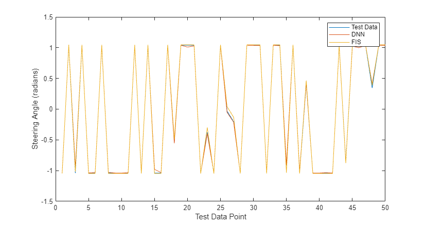
The DNN and FIS both reproduce the expected steering angles from the training data.

Explain Black-Box Model Using FIS

To explain the black-box model, first specify meaningful names for the MFs of each FIS. Doing so improves the interpretability of the FIS behavior.

mfNames = {...
    ["negative" "positive"], ...
    ["negative" "zero" "positive"], ...
    ["negativeLow" "negative" "positive" "positiveHigh"] ...
    };

for fisId = 1:numel(fisToutMF.FIS)
    for inId = 1:numel(fisToutMF.FIS(fisId).Inputs)
        numInputMFs = numel(fisToutMF.FIS(fisId).Inputs(inId).MembershipFunctions);
        names = mfNames{numInputMFs-1};
        for mfId = 1:numel(fisToutMF.FIS(fisId).Inputs(inId).MembershipFunctions)
            fisToutMF.FIS(fisId).Inputs(inId).MembershipFunctions(mfId).Name = names(mfId);
        end
    end

    numOutputMFs = numel(fisToutMF.FIS(fisId).Outputs(1).MembershipFunctions);
    names = mfNames{numOutputMFs-1};
    for mfId = 1:numOutputMFs
        fisToutMF.FIS(fisId).Outputs(1).MembershipFunctions(mfId).Name = names(mfId);
    end

end

View the FIS rules.

showRules(fisToutMF)

                         fis1Rules                                               fis2Rules                     
    ____________________________________________________    ___________________________________________________

    "Vy==negative & e1==negative => u1=positiveHigh (1)"    "r==negative & e2==negative => u2=negativeLow (1)" 
    "Vy==positive & e1==negative => u1=positive (1)"        "r==positive & e2==negative => u2=negative (1)"    
    "Vy==negative & e1==positive => u1=negative (1)"        "r==negative & e2==positive => u2=positiveHigh (1)"
    "Vy==positive & e1==positive => u1=negativeLow (1)"     "r==positive & e2==positive => u2=positive (1)"    

                         fis3Rules                                             fis4Rules                   
    ____________________________________________________    _______________________________________________

    "u1==negative & u2==negative => u3=positive (1)"        "u3==negative & u==negative => u4=negative (1)"
    "u1==positive & u2==negative => u3=positiveHigh (1)"    "u3==positive & u==negative => u4=positive (1)"
    "u1==negative & u2==positive => u3=negativeLow (1)"     "u3==negative & u==positive => u4=negative (1)"
    "u1==positive & u2==positive => u3=negative (1)"        "u3==positive & u==positive => u4=positive (1)"

                       fis5Rules                   
    _______________________________________________

    "u4==negative & d==negative => u*=negative (1)"
    "u4==positive & d==negative => u*=positive (1)"
    "u4==negative & d==positive => u*=negative (1)"
    "u4==positive & d==positive => u*=positive (1)"

You can make the following observations from the rule bases.

• Steering angle ${\mathit{u}}_1$ (output of fis1) is inversely proportional to lateral velocity (${\mathit{V}}_{\mathit{y}}$) and deviation (${\mathit{e}}_1$). For example, the first rule of fis1 describes that the steering angle ${\mathit{u}}_1$ is positiveHigh (high positive value) when the lateral velocity (${\mathit{V}}_{\mathit{y}}$) and deviation (${\mathit{e}}_1$) are both negative.

• Steering angle ${\mathit{u}}_2$ (output of fis2) is proportional to yaw angle rate ($\mathit{r}$) and relative yaw angle (${\mathit{e}}_2$). For example, the first rule of fis2 describes that the steering angle ${\mathit{u}}_2$ is negativeLow (low negative value) when the yaw angle rate ($\mathit{r}$) and relative yaw angle (${\mathit{e}}_2$) are both negative.

• Steering angles ${\mathit{u}}_1$ (output of fis1) and ${\mathit{u}}_2$ (output of fis2) have a negative correlation, that is, fis3 output ${\mathit{u}}_3$ increases when ${\mathit{u}}_1$ increases, whereas ${\mathit{u}}_3$ decreases when ${\mathit{u}}_2$ increases. Hence, the lateral deviation and yaw angle have opposite effects on the steering angle.

• The rule base of fis4 shows that the previous steering input $\mathit{u}$ has insignificant effect on the steering angle calculation. The output ${\mathit{u}}_4$ of fis4 uses similar linguistic variables as does the output of fis3.

• The measured disturbance $\mathit{d}$ also has insignificant effect on the steering angle calculation since the output ${\mathit{u}}_5$ of fis5 uses similar linguistic variables as does the output of fis4.

Hence, the rule bases of the FISs in the FIS tree describe the effects and relations between the input variables for steering calculation in the LKA system.

You can visualize each rule base using its control surface, which describes numerical mappings from the inputs to output according to the rule base.

figure
subplot(3,2,1)
gensurf(fisToutMF.FIS(1))
subplot(3,2,2)
gensurf(fisToutMF.FIS(2))
subplot(3,2,3)
gensurf(fisToutMF.FIS(3))
subplot(3,2,4)
gensurf(fisToutMF.FIS(4))
subplot(3,2,5)
gensurf(fisToutMF.FIS(5))

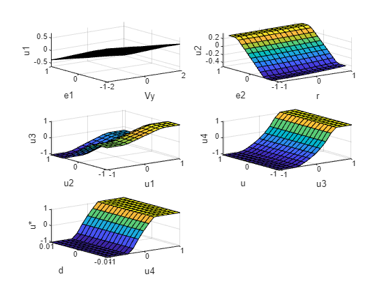
A fuzzy rule base provides linguistic relation between the inputs and output. The control surface augments this linguistic relation by adding numeric detail for input to output mapping.

Explain Run-Time Black-Box Predictions

The previous explanation of the black-box behavior describes the general relationships between the input observations and the resulting steering angle by interpreting the rule base of the fuzzy support system itself.

You can also use the support system to explain black-box outcomes generated in each control interval. The following diagram explains the parallel execution settings of the black-box model and the support system for run-time explanation of the black-box predictions.

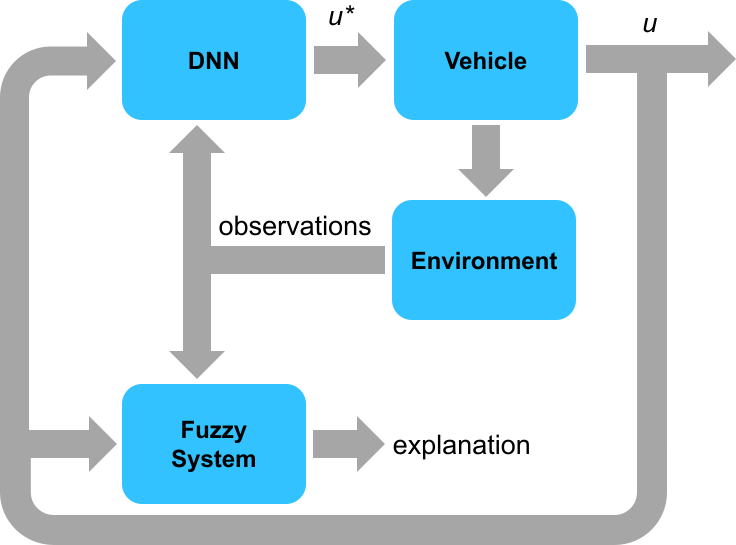
The black-box model and the support system run in parallel and use the same input values (observations) for output prediction. The prediction from black-box model drives environment changes, while the support system only explains the black-box predictions. For this example, the fuzzy support system includes the following components in the explanation for each control interval.

1. Current simulation time

2. Current input values

3. Steering angle outputs generated by the DNN black-box model and fuzzy support system

4. Fuzzy rules having the maximum firing strength from each FIS of the FIS tree.

The output data format for each control interval is as follows.

================ Simulation time: <t> sec ================
inputs: [v r e1 e2 u d], outputs: [u*(DNN) u*(fuzzy)] rad
Max strength rules:
    fis1: <rule description> 
    fis2: <rule description> 
    fis3: <rule description>
    fis4: <rule description> 
    fis5: <rule description>

The following simulation results explain the DNN model outputs in each control cycle using the fuzzy support system.

Initialize the vehicle state using the input from a test data point.

id = round(median(1:size(data.testInputData,1)));
x0 = data.testInputData(id,:);

Simulate the DNN and FIS with the same input data using the compareDNNWithFIS helper function.

[dnnOutputs,fisOutput] = compareDNNWithFIS(dnnLKA,fisToutMF,data,x0);

================ Simulation time: 0 sec ================
inputs: [0.0737824 -0.726656 -0.0161284 0.0484033 0.569496 -0.00256057], 
outputs: [1.01041 1.0472] rad
Max strength rules:
	fis1: Vy==positive & e1==negative => u1=positive (1)
	fis2: r==positive & e2==positive => u2=positive (1)
	fis3: u1==positive & u2==negative => u3=positiveHigh (1)
	fis4: u3==positive & u==negative => u4=positive (1)
	fis5: u4==positive & d==negative => u*=positive (1)
================ Simulation time: 0.1 sec ================
inputs: [1.2579 -0.532934 1.33827 0.119282 1.01041 -0.00256057], 
outputs: [-0.0654638 -0.114224] rad
Max strength rules:
	fis1: Vy==positive & e1==negative => u1=positive (1)
	fis2: r==positive & e2==positive => u2=positive (1)
	fis3: u1==positive & u2==positive => u3=negative (1)
	fis4: u3==negative & u==negative => u4=negative (1)
	fis5: u4==negative & d==negative => u*=negative (1)
================ Simulation time: 0.2 sec ================
inputs: [-0.338464 -0.23482 0.745212 0.222974 -0.0654638 -0.00256057], 
outputs: [-0.933683 -0.982878] rad
Max strength rules:
	fis1: Vy==positive & e1==negative => u1=positive (1)
	fis2: r==positive & e2==positive => u2=positive (1)
	fis3: u1==positive & u2==positive => u3=negative (1)
	fis4: u3==negative & u==negative => u4=negative (1)
	fis5: u4==negative & d==negative => u*=negative (1)
================ Simulation time: 0.3 sec ================
inputs: [-1.86933 -0.0209625 -0.862648 0.212142 -0.933683 -0.00256057], 
outputs: [-0.817988 -0.751812] rad
Max strength rules:
	fis1: Vy==negative & e1==negative => u1=positiveHigh (1)
	fis2: r==negative & e2==positive => u2=positiveHigh (1)
	fis3: u1==positive & u2==positive => u3=negative (1)
	fis4: u3==negative & u==negative => u4=negative (1)
	fis5: u4==negative & d==negative => u*=negative (1)
================ Simulation time: 0.4 sec ================
inputs: [-1.43016 0.0363023 -1.71046 0.0795596 -0.817988 -0.00256057], 
outputs: [0.067486 0.285178] rad
Max strength rules:
	fis1: Vy==negative & e1==negative => u1=positiveHigh (1)
	fis2: r==negative & e2==positive => u2=positiveHigh (1)
	fis3: u1==positive & u2==negative => u3=positiveHigh (1)
	fis4: u3==positive & u==negative => u4=positive (1)
	fis5: u4==positive & d==negative => u*=positive (1)
================ Simulation time: 0.5 sec ================
inputs: [0.518155 0.0163838 -0.959078 -0.0526409 0.067486 -0.00256057], 
outputs: [0.341617 0.307694] rad
Max strength rules:
	fis1: Vy==positive & e1==negative => u1=positive (1)
	fis2: r==negative & e2==negative => u2=negativeLow (1)
	fis3: u1==negative & u2==negative => u3=positive (1)
	fis4: u3==positive & u==negative => u4=positive (1)
	fis5: u4==positive & d==negative => u*=positive (1)
================ Simulation time: 0.6 sec ================
inputs: [1.43122 0.00176658 -0.0241615 -0.0985401 0.341617 -0.00256057], 
outputs: [0.2509 0.266469] rad
Max strength rules:
	fis1: Vy==positive & e1==negative => u1=positive (1)
	fis2: r==positive & e2==negative => u2=negative (1)
	fis3: u1==negative & u2==negative => u3=positive (1)
	fis4: u3==positive & u==negative => u4=positive (1)
	fis5: u4==positive & d==negative => u*=positive (1)
================ Simulation time: 0.7 sec ================
inputs: [1.16149 -0.000896733 0.439618 -0.075189 0.2509 -0.00256057], 
outputs: [0.0708356 0.0913793] rad
Max strength rules:
	fis1: Vy==positive & e1==negative => u1=positive (1)
	fis2: r==positive & e2==negative => u2=negative (1)
	fis3: u1==negative & u2==negative => u3=positive (1)
	fis4: u3==negative & u==negative => u4=negative (1)
	fis5: u4==positive & d==negative => u*=positive (1)
================ Simulation time: 0.8 sec ================
inputs: [0.440393 -0.00281434 0.429965 -0.0306668 0.0708356 -0.00256057], 
outputs: [-0.018147 0.00702747] rad
Max strength rules:
	fis1: Vy==positive & e1==negative => u1=positive (1)
	fis2: r==positive & e2==negative => u2=negative (1)
	fis3: u1==positive & u2==negative => u3=positiveHigh (1)
	fis4: u3==negative & u==negative => u4=negative (1)
	fis5: u4==positive & d==negative => u*=positive (1)
================ Simulation time: 0.9 sec ================
inputs: [-0.0839109 -0.00710326 0.246288 0.00320765 -0.018147 -0.00256057], 
outputs: [-0.0571112 -0.0431572] rad
Max strength rules:
	fis1: Vy==positive & e1==negative => u1=positive (1)
	fis2: r==positive & e2==negative => u2=negative (1)
	fis3: u1==positive & u2==negative => u3=positiveHigh (1)
	fis4: u3==negative & u==negative => u4=negative (1)
	fis5: u4==negative & d==negative => u*=negative (1)
================ Simulation time: 1 sec ================
inputs: [-0.302092 -0.0110731 0.0509452 0.0177286 -0.0571112 -0.00256057], 
outputs: [-0.0356867 -0.00903791] rad
Max strength rules:
	fis1: Vy==positive & e1==negative => u1=positive (1)
	fis2: r==positive & e2==positive => u2=positive (1)
	fis3: u1==positive & u2==negative => u3=positiveHigh (1)
	fis4: u3==negative & u==negative => u4=negative (1)
	fis5: u4==negative & d==negative => u*=negative (1)
================ Simulation time: 1.1 sec ================
inputs: [-0.258972 -0.012099 -0.0449731 0.0178176 -0.0356867 -0.00256057], 
outputs: [-0.0338398 -0.00862586] rad
Max strength rules:
	fis1: Vy==positive & e1==negative => u1=positive (1)
	fis2: r==positive & e2==positive => u2=positive (1)
	fis3: u1==positive & u2==negative => u3=positiveHigh (1)
	fis4: u3==negative & u==negative => u4=negative (1)
	fis5: u4==negative & d==negative => u*=negative (1)
================ Simulation time: 1.2 sec ================
inputs: [-0.159425 -0.01097 -0.091006 0.0109606 -0.0338398 -0.00256057], 
outputs: [-0.0138319 0.000404072] rad
Max strength rules:
	fis1: Vy==positive & e1==negative => u1=positive (1)
	fis2: r==positive & e2==positive => u2=positive (1)
	fis3: u1==positive & u2==negative => u3=positiveHigh (1)
	fis4: u3==negative & u==negative => u4=negative (1)
	fis5: u4==positive & d==negative => u*=positive (1)
================ Simulation time: 1.3 sec ================
inputs: [-0.0423529 -0.0105425 -0.0811233 0.00251846 -0.0138319 -0.00256057], 
outputs: [0.000331631 0.0269576] rad
Max strength rules:
	fis1: Vy==positive & e1==negative => u1=positive (1)
	fis2: r==positive & e2==negative => u2=negative (1)
	fis3: u1==positive & u2==negative => u3=positiveHigh (1)
	fis4: u3==negative & u==negative => u4=negative (1)
	fis5: u4==positive & d==negative => u*=positive (1)
================ Simulation time: 1.4 sec ================
inputs: [0.0361998 -0.0114349 -0.0471621 -0.00358271 0.000331631 -0.00256057], 
outputs: [0.0304953 0.0473974] rad
Max strength rules:
	fis1: Vy==positive & e1==negative => u1=positive (1)
	fis2: r==positive & e2==negative => u2=negative (1)
	fis3: u1==positive & u2==negative => u3=positiveHigh (1)
	fis4: u3==negative & u==negative => u4=negative (1)
	fis5: u4==positive & d==negative => u*=positive (1)
================ Simulation time: 1.5 sec ================
inputs: [0.0930044 -0.0110261 0.0178849 -0.0045736 0.0304953 -0.00256057], 
outputs: [0.00543881 0.0263823] rad
Max strength rules:
	fis1: Vy==positive & e1==negative => u1=positive (1)
	fis2: r==positive & e2==negative => u2=negative (1)
	fis3: u1==positive & u2==negative => u3=positiveHigh (1)
	fis4: u3==negative & u==negative => u4=negative (1)
	fis5: u4==positive & d==negative => u*=positive (1)
================ Simulation time: 1.6 sec ================
inputs: [0.0479659 -0.00916726 0.0247146 -0.00210616 0.00543881 -0.00256057], 
outputs: [-0.00489218 0.013721] rad
Max strength rules:
	fis1: Vy==positive & e1==negative => u1=positive (1)
	fis2: r==positive & e2==negative => u2=negative (1)
	fis3: u1==positive & u2==negative => u3=positiveHigh (1)
	fis4: u3==negative & u==negative => u4=negative (1)
	fis5: u4==positive & d==negative => u*=positive (1)
================ Simulation time: 1.7 sec ================
inputs: [0.00396816 -0.00833844 0.0109447 -7.63103e-05 -0.00489218 -0.00256057], 
outputs: [-0.0103413 0.0106303] rad
Max strength rules:
	fis1: Vy==positive & e1==negative => u1=positive (1)
	fis2: r==positive & e2==negative => u2=negative (1)
	fis3: u1==positive & u2==negative => u3=positiveHigh (1)
	fis4: u3==negative & u==negative => u4=negative (1)
	fis5: u4==positive & d==negative => u*=positive (1)
================ Simulation time: 1.8 sec ================
inputs: [-0.018166 -0.0089212 -0.00744726 0.000300261 -0.0103413 -0.00256057], 
outputs: [-0.00482928 0.0185661] rad
Max strength rules:
	fis1: Vy==positive & e1==negative => u1=positive (1)
	fis2: r==positive & e2==negative => u2=negative (1)
	fis3: u1==positive & u2==negative => u3=positiveHigh (1)
	fis4: u3==negative & u==negative => u4=negative (1)
	fis5: u4==positive & d==negative => u*=positive (1)
================ Simulation time: 1.9 sec ================
inputs: [-0.0108874 -0.0104442 -0.0119736 -0.00044273 -0.00482928 -0.00256057], 
outputs: [0.00649286 0.0270567] rad
Max strength rules:
	fis1: Vy==positive & e1==negative => u1=positive (1)
	fis2: r==positive & e2==negative => u2=negative (1)
	fis3: u1==positive & u2==negative => u3=positiveHigh (1)
	fis4: u3==negative & u==negative => u4=negative (1)
	fis5: u4==positive & d==negative => u*=positive (1)
================ Simulation time: 2 sec ================
inputs: [0.0102737 -0.0112775 0.00120233 -0.000692395 0.00649286 -0.00256057], 
outputs: [0.00606815 0.023241] rad
Max strength rules:
	fis1: Vy==positive & e1==negative => u1=positive (1)
	fis2: r==positive & e2==negative => u2=negative (1)
	fis3: u1==positive & u2==negative => u3=positiveHigh (1)
	fis4: u3==negative & u==negative => u4=negative (1)
	fis5: u4==positive & d==negative => u*=positive (1)
================ Simulation time: 2.1 sec ================
inputs: [0.0123836 -0.0105726 0.00956554 0.000135917 0.00606815 -0.00256057], 
outputs: [-0.00548606 0.0132276] rad
Max strength rules:
	fis1: Vy==positive & e1==negative => u1=positive (1)
	fis2: r==positive & e2==negative => u2=negative (1)
	fis3: u1==positive & u2==negative => u3=positiveHigh (1)
	fis4: u3==negative & u==negative => u4=negative (1)
	fis5: u4==positive & d==negative => u*=positive (1)
================ Simulation time: 2.2 sec ================
inputs: [-0.00638756 -0.00962136 -0.00104885 0.000793332 -0.00548606 -0.00256057], 
outputs: [-0.0101493 0.0127077] rad
Max strength rules:
	fis1: Vy==positive & e1==negative => u1=positive (1)
	fis2: r==positive & e2==negative => u2=negative (1)
	fis3: u1==positive & u2==negative => u3=positiveHigh (1)
	fis4: u3==negative & u==negative => u4=negative (1)
	fis5: u4==positive & d==negative => u*=positive (1)
================ Simulation time: 2.3 sec ================
inputs: [-0.0150607 -0.00993626 -0.0145728 0.000219598 -0.0101493 -0.00256057], 
outputs: [-0.000622749 0.0224691] rad
Max strength rules:
	fis1: Vy==positive & e1==negative => u1=positive (1)
	fis2: r==positive & e2==negative => u2=negative (1)
	fis3: u1==positive & u2==negative => u3=positiveHigh (1)
	fis4: u3==negative & u==negative => u4=negative (1)
	fis5: u4==positive & d==negative => u*=positive (1)
================ Simulation time: 2.4 sec ================
inputs: [0.00129175 -0.0109741 -0.0100013 -0.000752014 -0.000622749 -0.00256057], 
outputs: [0.00826702 0.0272876] rad
Max strength rules:
	fis1: Vy==positive & e1==negative => u1=positive (1)
	fis2: r==positive & e2==negative => u2=negative (1)
	fis3: u1==positive & u2==negative => u3=positiveHigh (1)
	fis4: u3==negative & u==negative => u4=negative (1)
	fis5: u4==positive & d==negative => u*=positive (1)
================ Simulation time: 2.5 sec ================
inputs: [0.0180957 -0.0110403 0.00564719 -0.000665084 0.00826702 -0.00256057], 
outputs: [0.00268267 0.0195868] rad
Max strength rules:
	fis1: Vy==positive & e1==negative => u1=positive (1)
	fis2: r==positive & e2==negative => u2=negative (1)
	fis3: u1==positive & u2==negative => u3=positiveHigh (1)
	fis4: u3==negative & u==negative => u4=negative (1)
	fis5: u4==positive & d==negative => u*=positive (1)
================ Simulation time: 2.6 sec ================
inputs: [0.00964099 -0.00996295 0.00814148 0.000300946 0.00268267 -0.00256057], 
outputs: [-0.00864567 0.0113769] rad
Max strength rules:
	fis1: Vy==positive & e1==negative => u1=positive (1)
	fis2: r==positive & e2==negative => u2=negative (1)
	fis3: u1==positive & u2==negative => u3=positiveHigh (1)
	fis4: u3==negative & u==negative => u4=negative (1)
	fis5: u4==positive & d==negative => u*=positive (1)
================ Simulation time: 2.7 sec ================
inputs: [-0.0106986 -0.00937355 -0.00624473 0.000612801 -0.00864567 -0.00256057], 
outputs: [-0.00803808 0.0154329] rad
Max strength rules:
	fis1: Vy==positive & e1==negative => u1=positive (1)
	fis2: r==positive & e2==negative => u2=negative (1)
	fis3: u1==positive & u2==negative => u3=positiveHigh (1)
	fis4: u3==negative & u==negative => u4=negative (1)
	fis5: u4==positive & d==negative => u*=positive (1)
================ Simulation time: 2.8 sec ================
inputs: [-0.0111989 -0.0101628 -0.0149538 -0.000228281 -0.00803808 -0.00256057], 
outputs: [0.00356137 0.0254181] rad
Max strength rules:
	fis1: Vy==positive & e1==negative => u1=positive (1)
	fis2: r==positive & e2==negative => u2=negative (1)
	fis3: u1==positive & u2==negative => u3=positiveHigh (1)
	fis4: u3==negative & u==negative => u4=negative (1)
	fis5: u4==positive & d==negative => u*=positive (1)
================ Simulation time: 2.9 sec ================
inputs: [0.00883551 -0.0110872 -0.00433248 -0.000913484 0.00356137 -0.00256057], 
outputs: [0.00806062 0.0257676] rad
Max strength rules:
	fis1: Vy==positive & e1==negative => u1=positive (1)
	fis2: r==positive & e2==negative => u2=negative (1)
	fis3: u1==positive & u2==negative => u3=positiveHigh (1)
	fis4: u3==negative & u==negative => u4=negative (1)
	fis5: u4==positive & d==negative => u*=positive (1)

Plot the DNN and FIS outputs.

plotValidationResults(data.Ts,dnnOutputs,fisOutput)

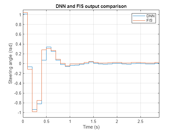
As expected, the fuzzy support system produces similar steering angle outputs as compared to the DNN black-box model.

Explanation Using Fuzzy Rule Inference

You can further explore the decision-making process of a FIS in the tree using its rule inference viewer. For example, the following simulation shows rule inference process of fis1 of the FIS tree.

fisIndex = 1;
showRuleInference(data,fisToutMF,fisIndex,x0)

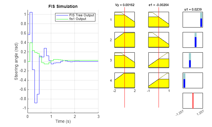
The left plot shows the output pattern of fis1 as compared to the overall FIS tree output. The right plot shows individual rule activations of fis1 in each control cycle.

FIS Tree Data Propagation

Finally, you can also visualize how each FIS contributes to the decision-making process for a given set of input values. The following example shows output propagation in the FIS tree for a test input vector.

[~,~,fisIns,fisOuts] = evaluateFISTree(fisToutMF,[x0(1) x0(3) x0(2) x0(4:6)]);
fisTwithIOValues = updateLabelsWithIOValues(fisToutMF,fisIns,fisOuts);

showFISTree(fisTwithIOValues,0.85)

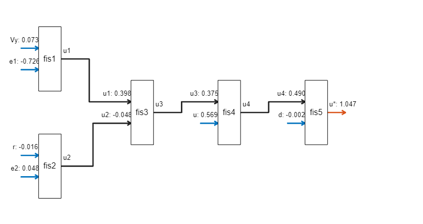
For this combination of input values, the output of fis1 dominates over the fis2 output, which indicates that lateral displacement and its rate contribute more to the overall output value.

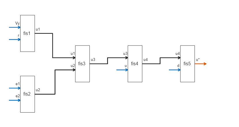
Conclusion

You can further improve the performance of the support fuzzy system by using:

• Additional input MFs

• Continuous MFs for smooth variations in outputs

• More training data, and

• Different configurations of the FIS tree, as shown in the following figure

showOtherBlackBoxFISTrees(data)

Example 1

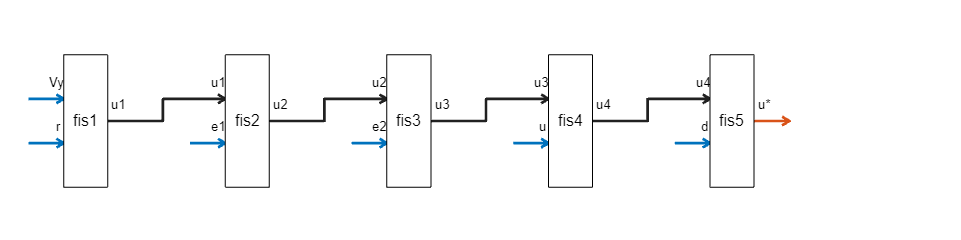
Example 2

Different tuning methods with different random number generation seeds may also improve the optimization of the support system.

You can also intuitively update each individual FIS rule base to check possible variations in output generation to further improve the performance of the support system.

Helper Functions

function fis = constructFIS(name,numMFs,in1range,in2range,outrange,in1,in2,out)
% Construct a Sugeno FIS.

fis = sugfis('Name',name);
numOutputMFs = numMFs^2;
fis = addInput(fis,in1range,'Name',in1,'NumMFs',numMFs);
fis = addInput(fis,in2range,'Name',in2,'NumMFs',numMFs);
for ct = 1:2
    fis.Inputs(ct).MembershipFunctions(1).Type = 'linzmf';
    fis.Inputs(ct).MembershipFunctions(end).Type = 'linsmf';
    numMFs = length(fis.Inputs(ct).MembershipFunctions);
end
fis = addOutput(fis,outrange,'Name',out,'NumMFs',numOutputMFs);
range = 1:numMFs;
[in1,in2] = ndgrid(range,range);
rules = [in1(:) in2(:) ones(numOutputMFs,3)];
fis = addRule(fis,rules);
end

function [rms,yFIS] = calculateRMS(fis,x,y)
% Evaluate the FIS using the specified input data and calculate the RMS error
% the simulated and reference outputs.

options = evalfisOptions;
options.EmptyOutputFuzzySetMessage = 'none';
options.NoRuleFiredMessage = 'none';
options.OutOfRangeInputValueMessage = 'none';

yFIS = evalfis(fis,x,options);
e = yFIS - y;
rms = sqrt(mean(e.*e));
end

function showRules(fisT)
% Display rule bases of the FISs in a FIS tree as tables.

fis1Rules = [fisT.FIS(1).Rules.Description]';
fis2Rules = [fisT.FIS(2).Rules.Description]';
fis3Rules = [fisT.FIS(3).Rules.Description]';
fis4Rules = [fisT.FIS(4).Rules.Description]';
fis5Rules = [fisT.FIS(5).Rules.Description]';

disp(table(fis1Rules,fis2Rules))
disp(table(fis3Rules,fis4Rules))
disp(table(fis5Rules))
end

function [uHistoryDNN,uHistoryFIS] = compareDNNWithFIS(dnnLKA,fisToutMF,data,x0)
% Compares DNN and FIS tree model.

xHistoryDNN = repmat(x0(1:4),data.Tsteps+1,1);
uHistoryDNN = zeros(data.Tsteps,1);
uHistoryFIS = zeros(data.Tsteps,1);

lastMV = x0(5);
d = x0(6);
for k = 1:data.Tsteps
    % Obtain plant output measurements, which correspond to the plant outputs.
    xk = xHistoryDNN(k,:)';
    % Predict the next move using the trained deep neural network.
    in = [xk',lastMV,d];
    ukDNN = predict(dnnLKA,in);
    % Predict the next move using the trained fuzzy system.
    tmp = in(2); in(2) = in(3); in(3) = tmp; % config 1
    [ukFIS,maxRules] = evaluateFISTree(fisToutMF,in);
    % Store the control action and update the last MV for the next step.
    uHistoryDNN(k,:) = ukDNN;
    uHistoryFIS(k,:) = ukFIS;
    lastMV = ukDNN;
    % Update the state using the control action.
    xHistoryDNN(k+1,:) = (data.A*xk + data.B*[ukDNN;d])';

    % Explanations/diagnostics
    fprintf('\n================ Simulation time: %g sec ================',...
        (k-1)*data.Ts);
    fprintf('\ninputs: [%g %g %g %g %g %g], \noutputs: [%g %g] rad', ...
        in(1),in(2),in(3),in(4),in(5),in(6),ukDNN,ukFIS);
    fprintf('\nMax strength rules:');
    fprintf('\n\tfis1: %s\n\tfis2: %s\n\tfis3: %s\n\tfis4: %s\n\tfis5: %s', ...
        maxRules(1),maxRules(2),maxRules(3),maxRules(4),maxRules(5));
end

end

function [y,maxRules,fisIns,fisOuts] = evaluateFISTree(fisT,x)
% Evaluates FIS tree with the specified input values.

options = evalfisOptions;
options.OutOfRangeInputValueMessage = 'none';
options.NoRuleFiredMessage = 'none';
options.EmptyOutputFuzzySetMessage = 'none';

numFIS = numel(fisT.FIS);
fisIns = zeros(numFIS,2);

fisIns(1,:) = x(1:2);
[y1,~,~,~,rfs1] = evalfis(fisT.FIS(1),x(1:2),options);
fisIns(2,:) = x(3:4);
[y2,~,~,~,rfs2] = evalfis(fisT.FIS(2),x(3:4),options);
fisIns(3,:) = [y1 y2];
[y3,~,~,~,rfs3] = evalfis(fisT.FIS(3),[y1 y2],options);
fisIns(4,:) = [y3 x(5)];
[y4,~,~,~,rfs4] = evalfis(fisT.FIS(4),[y3 x(5)],options);
fisIns(5,:) = [y4 x(6)];
[y,~,~,~,rfs5] = evalfis(fisT.FIS(5),[y4 x(6)],options);

fisOuts = [y1 y2 y3 y4 y];

[~,id1] = sort(rfs1,'descend');
[~,id2] = sort(rfs2,'descend');
[~,id3] = sort(rfs3,'descend');
[~,id4] = sort(rfs4,'descend');
[~,id5] = sort(rfs5,'descend');

maxRules = [...
    fisT.FIS(1).Rules(id1(1)).Description; ...
    fisT.FIS(2).Rules(id2(1)).Description; ...
    fisT.FIS(3).Rules(id3(1)).Description; ...
    fisT.FIS(4).Rules(id4(1)).Description; ...
    fisT.FIS(5).Rules(id5(1)).Description ...    
    ];
end

function plotValidationResults(Ts,uDNN,uFIS)
% Plot validation results of the DNN and FIS tree model.
figure

% Plot output steering angles of DNN and FIS.
Tu  = ((0:(size(uDNN,1))-1)*Ts)';
stairs(Tu,uDNN);
title('DNN and FIS output comparison')
xlabel('Time (s)')
ylabel('Steering angle (rad)')
axis([0 Tu(end) -1.1 1.1]);
hold on
stairs(Tu,uFIS);
legend('DNN','FIS')
grid on;
hold off

pause(0.1)
end