Identify Delay Using Transient-Response Plots
You can use transient-response plots to estimate the input delay, or dead time, of linear systems. Input delay represents the time it takes for the output to respond to the input.
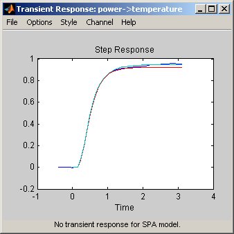
In the System Identification app: To view the transient response plot, select the Transient resp check box in the System Identification app. For example, the following step response plot shows a time delay of about 0.25 s before the system responds to the input.
Step Response Plot
At the command line: You can use impulseplot to plot the impulse response. The time delay is equal to the
first positive peak in the transient response magnitude that is greater than the
confidence region for positive time values.
For example, the following commands create an impulse-response plot with a 1-standard-deviation confidence region:
load dry2
ze = dry2(1:500);
opt = impulseestOptions('RegularizationKernel','TC');
sys = impulseest(ze,40,opt);
h = impulseplot(sys);
showConfidence(h,1);
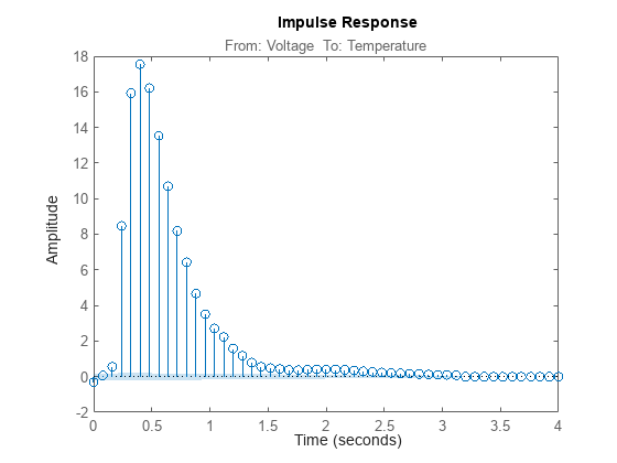
The resulting figure shows that the first positive peak of the response magnitude, which is greater than the confidence region for positive time values, occurs at 0.24 s.
Instead of using showConfidence, you can plot the
confidence interval interactively, by right-clicking on the plot and selecting Characteristics > Confidence Region.